Creating Your First Calculated Item

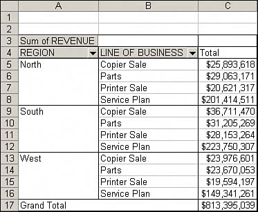
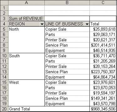
As you learned at the beginning of this chapter, a calculated item is essentially a row of data you add by performing a calculation on the other rows in the same field. Therefore, it makes sense that you must first select the field where you want to add your calculated item.

NOTE

As you go through this section, keep in mind that grouping items can give you an effect similar to that of creating a calculated item. Indeed, in many cases, grouping would be a great alternative to using calculated items. Chapter 5, "Controlling the Way You View Your Pivot Data," covers grouping in detail.

In the pivot table shown in Figure 6.18, you see totals for copier sales and printer sales under the Line of Business field. You need to group both of these data items into a calculated item called Equipment.

Figure 6.18. You want to add a new data item called Equipment that will represent the sum of copier sales and printer sales.

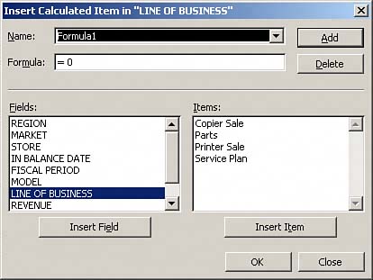
Place your cursor on any data item with the Line of Business field, click the PivotTable icon in the PivotTable toolbar, and select Formulas, Calculated Item. This activates the Insert Calculated Item dialog box shown in Figure 6.19.

Figure 6.19. The Insert Calculated Item dialog box will assist you in creating your calculated item.

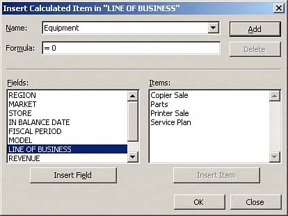
Notice that the top of the dialog box identifies which field you are working with. In this case, it is the Line of Business field. Also, notice the list box that contains all the items in the Line of Business field. Your goal is to give your calculated item a name and then build its formula by selecting the combination of data items and operators that will provide you the metric you are looking for.

As you can see in Figure 6.20, you will first name your calculated item Equipment.

Figure 6.20. Give your calculated item a descriptive name.

As mentioned before, the formula input box contains "= 0" by default. Ensure that you delete the zero before continuing with your formula.

Next, go to the Items list and double-click on the Copier Sale item. Then enter a plus sign (+) to signify that you will be adding this item to something. Finish your formula by double-clicking on the Printer Sale item in the Items list box.

At this point, your dialog box should look similar to the one shown in Figure 6.21. Here's your full formula:

Figure 6.21. You have successfully added a calculated item to your pivot table.

= 'Copier Sale' + 'Printer Sale'

This will give you the calculated item you need. Click OK to activate your new calculated item.

Now you can hide Copier Sale and Printer Sale, leaving the three distinct pivot items shown in Figure 6.22. Keep in mind that you can also change the settings on this new data item just as you would any other (for example, you can change the format or the color).

Figure 6.22. Hiding the Copier Sale and Printer Sale items gives you three distinct items and corrects the grand total.

CAUTION

If you don't hide the data items you used to create your calculated item, your grand totals and subtotals may double-count your units of measure (revenue, gallons, and so on). Compare the grand total in Figure 6.21 to the one in Figure 6.22.

CASE STUDY: Creating a Mini-Dashboard

You need to create a mini-dashboard that shows two key variances for each store:

• The current fiscal period versus the same period last year

• The last three fiscal period averages versus the same three last year

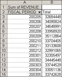
Figure 6.23 shows the data source you will be working with. Given the amount of data in your source table and the possibility that this will be a recurring exercise, you decide to build the dashboard with a pivot table.

Figure 6.23. Using a pivot table will give you the flexibility to update your dashboard report without re-creating it.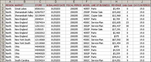

Create the initial pivot table as shown in Figure 6.24 by placing the Fiscal Period field in the row area and Revenue field in the data area.

Figure 6.24. The initial pivot table is basic, showing you revenue by fiscal period.

The first metric you need is the current fiscal period versus the same period last year. You will need to add a calculated item that uses the following formula:

Fiscal Period 200404 Fiscal Period 200304

Place your cursor on any data item under the Fiscal Period field and then click the PivotTable icon in the PivotTable toolbar. Next, select Formulas, Calculated Item. This activates the Insert Calculated Item dialog box. Name your new item Current PD vs. Last PD.

Delete the zero that appears in the Formula input box and then follow these steps:

1.	Double-click on the 200404 item.
2.	Enter a division sign (/).
3.	Double-click on the 200304 item.
4.	Enter -1.

At this point, your dialog box should look similar to the one shown in Figure 6.25. You can now click OK to add your new item.

Figure 6.25. You have successfully created the formula for your first metric (the current fiscal period versus the same period last year).

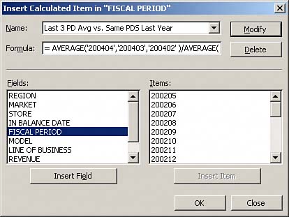
Next, you need to create a calculated item for the last three fiscal period averages versus the same three averages last year. The calculation for this metric is as follows:

Average('200404','200403','200402') / Average('200304','200303','200302') - 1

Place your cursor on any data item under the Fiscal Year field and activate the Insert Calculated Item dialog box. Then name your new item Last 3 PD Avg vs. Same PDS Last Year.

Delete the zero that appears in the Formula input box and then follow these steps:

1.	Enter =Average(.
2.	Double-click on the 200404 item and then enter a comma.
3.	Double-click on the 200403 item and then enter a comma.
4.	Double-click on the 200402 item.
5.	Enter )/Average(.
6.	Double-click on the 200304 item and then enter a comma.
7.	Double-click on the 200303 item and then enter a comma.
8.	Double-click on the 200302 item.
9.	Enter )-1.

Figure 6.26 gives you a good idea how this formula will look in your dialog box.

Figure 6.26. Your second formula uses six data items and two Average functions.

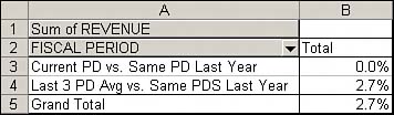
NOTE

Notice that you are using the Average function in this example. When building formulas in calculated fields or calculated items, you can use any worksheet function that does not require cell references or defined names as arguments.

Now hide all the data items in the Fiscal Year field except for the two calculated items you just created. Then change the calculated item values to percentage format. At this point, your pivot table should look like the one shown in Figure 6.27.

Figure 6.27. After hiding the data items you don't need and formatting the data in percentage format, you can see your dashboard starting to come together.

Add the Store field to the row field of your pivot table and drag Fiscal Period on top of Total, as shown in Figure 6.28.

Figure 6.28. Add the Store field and change the orientation of your calculated items to columnar.

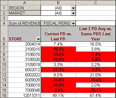
The last step in creating your mini-dashboard is to apply conditional formatting to your pivot table. Follow these steps:

1.	Select all the cells that contain your data area and apply conditional formatting to those cells.
2.	Go up to the application menu bar and select Format, Conditional Formatting.
3.	Set your condition to show: Cell Value is, less than, 0.
4.	Click the Format button and change the font and pattern colors to your liking.
5.	Click OK to apply your new format.

As you can see in Figure 6.29, conditional formatting provides for dynamic highlighting of problem areas, which adds another level of functionality to your pivot table report. Your mini-dashboard is ready for distribution!

Figure 6.29. You have successfully created your dashboard!

If you need to see this same dashboard next fiscal period, all you have to do is slightly alter your formulas and refresh your pivot table.