11.3 Layer 2 LAN Switch
11.3 Layer 2 LAN Switch
11.3.1 Layer 2 LAN Switch Features
There is literally an ever-expanding number of features being incorporated into Ethernet switches. These features range from providing such basic functions as port and segment switching to methods developed by some vendors to prevent erroneous frames from being transferred through the switch in a cut-through mode of operation. In this section we review 19 distinct switch features, as summarized in alphabetical order in Table 11.2.
| Feature | Requirement | Vendor A | Vendor B |
|---|---|---|---|
| Address table size support: | |||
| Addresses/port | |||
| Addresses/switch | |||
| Aging settings | |||
| Architecture: | |||
| ASIC based | |||
| CISC based | |||
| RISC based | |||
| Auto-negotiation ports | |||
| Backplane transfer capacity | |||
| Error prevention | |||
| Fat pipe and trunk group | |||
| Filtering/forwarding rate support: | |||
| Filtering rate | |||
| Forwarding rate | |||
| Flow control: | |||
| Backpressure | |||
| Software drivers | |||
| 802.3x flow control | |||
| No control | |||
| Full-duplex port operation | |||
| Jabber control | |||
| Latency | |||
| Management | |||
| Mirrored port | |||
| Module insertion | |||
| Port buffer size | |||
| Port module support | |||
| Spanning tree support | |||
| Switch type: | |||
| Port-based switch | |||
| Segment-based switch | |||
| Switching mode: | |||
| Cut-through | |||
| Store and forward | |||
| Hybrid | |||
| Virtual LAN support: | |||
| Port based | |||
| MAC based | |||
| Layer 3 based | |||
| Rule based |
The table of features presented was constructed not only to list features you should note, but, in addition, as a mechanism to facilitate the evaluation of switches. That is, you can indicate your requirement for a particular feature and then note whether or not that requirement can be satisfied by different vendor products by replacing "Vendor A" and "Vendor B" by the names of switches you are evaluating. By duplicating this table, you can extend the two right-most columns to evaluate more than two products. As we examine each feature listed in Table 11.2, our degree of exploration will be based on whether or not the feature was previously described. If the feature was previously described in this chapter, we will limit our discussion to a brief review of the feature. Otherwise , we will discuss its operation in considerable detail.
11.3.1.1 Address Table Size Support
The ability of a switch to correctly forward packets to their intended recipient depends on the use of address tables. Similarly, the capability of a switch to support a defined number of workstations depends on the number of entries that can be placed in its address table. Thus, the address table size can be viewed as a constraint that affects the ability of a switch to support network devices.
There are two address table sizes you may have to consider: the number of addresses supported per port and the number of addresses supported per switch. The first address table constraint is only applicable for ports that support the connection of network segments. In comparison, the total number of addresses recognized per switch represents a constraint that affects the entire switch. Many Ethernet switches support up to 1024 addresses per port for segment-based support. Such switches may only support a total of 8192 addresses per switch. This means that a 16-port switch with eight fully populated segments could not support the use of the eight remaining ports as the switch would run out of address table entries. Thus, it is important to consider the number of addresses supported per port and per switch as well as match such data against the anticipated requirements.
11.3.1.2 Aging Settings
MAC addresses and their associated port are stored with a timestamp value. This provides the bridge with the ability to purge old entries to make room for new entries in the port-address table. Because a switch is a multi-port bridge, it also uses a timer to purge old entries from its port-address table. Some switches provide users with the ability to set the aging time within a wide range of values or to disable aging. Other switches have a series of predefined aging values from which a user can select.
11.3.1.3 Architecture
As previously noted, there are three basic methods used to construct LAN switches. Those methods include a bus-based design, shared memory, and a crossbar matrix design. The first two methods are typically simpler and less expensive to implement than a crossbar design. However, the crossbar design is more scalable as well as provides a true parallel switching capability.
11.3.1.4 Auto-Negotiation Ports
To provide a mechanism to migrate from 10 Mbps to 100 Mbps, National Semiconductor developed a chip set known as Nway; it provides an automatic data rate sensing capability as part of an auto-negotiation function. This capability enables a switch port to support either a 10- or 100-Mbps Ethernet attachment to the port; however, this feature only works when cabled to a 10/100-Mbps network adapter card. You may otherwise have to use the switch console to configure the operating rate of the port or the port may be fixed to a predefined operating rate.
11.3.1.5 Backplane Transfer Capacity
The backplane transfer capacity of a switch provides you with the ability to determine how well the device can support a large number of simultaneous cross-connections, as well as its ability to perform flooding. For example, consider a 64-port 10BASE-T switch with a backplane transfer capacity of 400 Mbps. Because the switch can support a maximum of 64/2 or 32 cross-connects, the switch's backplane must provide at least a 32 * 10 Mbps or 320 Mbps transfer capacity. However, when it encounters an unknown destination address on one port, the switch will output or flood the packet onto all ports other than the port on which the frame was received. Thus, to operate in a non-blocked mode to effect flooding, the switch must have a buffer transfer capacity of 64 * 10 Mbps, or 640 Mbps.
11.3.1.6 Error Prevention
Some switch designers recognize that the majority of runt frames (frames improperly terminated ) result from a collision occurring during the time it takes to read the first 64 bytes of the frame. On a 10-Mbps Ethernet LAN, this is equivalent to a time of 51.2 ¼ s. In a cut-through switch environment when latency is minimized, it becomes possible to pass runt frames to the destination. To preclude this from happening, some switch designers permit the user to introduce a 51.2- ¼ s delay that provides sufficient time for the switch to verify that the frame is of sufficient length to have a high degree of probability that it is not a runt frame. Other switches that operate in the cut-through mode may simply impose a 51.2- ¼ s delay at 10 Mbps to enable this error prevention feature. Regardless of the method used, the delay is only applicable to cut-through switches that support LAN segments, as single user ports do not generate collisions.
11.3.1.7 Fat Pipe and Trunk Group
A fat pipe is a term used to reference a high-speed port. When 10BASE-T switches were first introduced, the term actually referenced a group of two or more ports operating as an entity. Today, a fat pipe can reference a 100-Mbps port on a switch primarily consisting of 10-Mbps operating ports or a 155-Mbps ATM port on a 10/100 or 100-Mbps switch. In addition, some vendors retain the term "fat pipe" as a reference to a group of ports operating as an entity while other vendors use the term "trunk group" to represent a group of ports that function as an entity. However, to support a grouping of ports operating as a common entity requires the interconnected switches to be obtained from the same company as the method used to group ports is proprietary.
11.3.1.8 Filtering and Forwarding Rate Support
The ability of a switch to interpret a number of frame destination addresses during a defined time interval is referred to as its filtering rate. In comparison, the number of frames that must be routed through a switch during a predefined period of time is referred to as the forwarding rate. Both the filtering and forwarding rates govern the performance level of a switch with respect to its ability to interpret and route frames. When considering these two metrics, it is important to understand the maximum frame rate on an Ethernet LAN; this was discussed earlier in this book.
11.3.1.9 Flow Control
Flow control represents the orderly regulation of transmission. In a switched network environment there are a number of situations for which flow control can be used to prevent the loss of data and subsequent retransmissions which can create a cycle of lost data followed by retransmissions. The most common cause of lost data results from a data rate mismatch between source and destination ports. For example, consider a server connected to a switch via a Fast Ethernet 100-Mbps connection that responds to a client query when the client is connected to a switch port at 10 Mbps. Without the use of a buffer within the switch, this speed mismatch would always result in the loss of data. Through the use of a buffer, data can be transferred into the switch at 100 Mbps and transferred out at 10 Mbps. However, because the input rate is ten times the output rate, the buffer will rapidly fill. In addition, if the server is transferring a large quantity of data, the buffer could overflow, resulting in subsequent data sent to the switch being lost. Thus, unless the length of the buffer is infinite, an impossible situation, there would always be some probability that data could be lost.
Another common cause of lost data is when multiple source port inputs are contending for access to the same destination port. If each source and destination port operates at the same data rate, then only two source ports contending for access to the same destination port can result in the loss of data. Thus, a mechanism is required to regulate the flow of data through a switch. That mechanism is flow control.
All Ethernet switches this author is familiar with have either buffers in each port or centralized memory that functions as a buffer. The key difference between switch buffers is in the amount of memory used. Some switches have 128K, 256 Kbytes, or even 1 or 2 Mbytes per port, whereas other switches may support the temporary storage of 10 or 20 full-length Ethernet frames. To prevent buffer overflow, four techniques are used: backpressure, proprietary software, IEEE 802.3x flow control, and no control. Thus, lets examine each technique.
11.3.1.10 Backpressure
Backpressure represents a technique by which a switch generates a false collision signal. In actuality, the switch port operates as if it detected a collision and initiates the transmission of a jam pattern. The jam pattern consists of 32 to 48 bits that can have any value other than the CRC value that corresponds to any partial frame transmitted before the jam.
The transmission of the jam pattern ensures that the collision lasts long enough to be detected by all stations on the network. In addition, the jam signal serves as a mechanism to cause non-transmitting stations to wait until the jam signal ends prior to attempting to transmit, thus alleviating additional potential collisions from occurring. Although the jam signal temporarily stops transmission, enabling the contents of buffers to be output, the signal also adversely affects all stations connected to the port. Thus, a network segment consisting of a number of stations connected to a switch port would result in all stations having their transmission capability suspended even when just one station was directing traffic to the switch.
Backpressure is commonly implemented based upon the level of buffer memory used. When buffer memory is filled to a predefined level, that level serves as a threshold for the switch to generate jam signals. Then, once the buffer is emptied beyond another lower level, that level serves as a threshold to disable backpressure operations.
11.3.1.11 Proprietary Software Drivers
Software drivers enable a switch to directly communicate with an attached device. This enables the switch to enable and disable the station's transmission capability. Currently, software drivers are available as a NetWare Loadable Module (NLM) for NetWare servers, and may be available for Windows 2000 by the time you read this book.
11.3.1.12 IEEE 802.3x Flow Control
During 1997, the IEEE standardized a method that provides flow control on full-duplex Ethernet connections. To provide this capability, a special "Pause" frame was defined that is transmitted by devices that want to stop the flow of data from the device at the opposite end of the link.
Figure 11.18 illustrates the format of the Pause frame. Because a full-duplex connection has a device on each end of the link, the use of a predefined destination address and operation code (OpCode) defines the frame as a Pause frame. The value following the OpCode defines the time in terms of slot times that the transmitting device wants its partner to pause. This initial pause time can be extended by additional Pause frames containing new slot time values or canceled by another Pause frame containing a zero slot time value. The Pad field shown at the end of the Pause frame must have each of its 42 bytes set to zero.
| Destination | Source | Type | OpCod | Pause time | Pad |
Figure 11.18: The IEEE 802.3x Pause Frame
Under the 802.3x standard, the use of Pause frames is auto-negotiated on copper media and can be manually configured for use on fiber links. The actual standard does not require a device capable of sending a Pause frame to actually do so. Instead, it provides a standard for recognizing a Pause frame as well as a mechanism for interpreting the contents of the frame so a receiver can correctly respond to it.
The IEEE 802.3x flow control standard is applicable to all versions of Ethernet from 10 Mbps to 1 Gbps; however, the primary purpose of this standard is to enable switches to be manufactured with a minimal amount of memory. By supporting the IEEE 802.3x standard, a switch with a limited amount of memory can generate Pause frames to regulate inbound traffic instead of having to drop frames when its buffer is full.
11.3.1.13 No Control
Many switch vendors rely on the fact that the previously described traffic patterns that can result in buffers overflowing and the loss of data have a relatively low probability of occurrence for any significant length of time. In addition, upper layers of the OSI Reference Model will retransmit lost packets. Thus, many switch vendors rely on the use of memory buffers and do not incorporate flow control into their products. Whether or not this is an appropriate solution will depend on the traffic you anticipate flowing through the switch.
11.3.1.14 Full-Duplex Port Operation
If a switch port only supports the connection of one station, a collision can never occur. Recognizing this fact, most Ethernet switch vendors now support full-duplex or bi-directional traffic flow by using two of the four wire connections for 10BASE-T for transmission in the opposite direction. Full-duplex support is available for 10BASE-T, Fast Ethernet, and Gigabit Ethernet connections. Because collisions can occur on a segment, switch ports used for segment-based switching cannot support full-duplex transmission.
In addition to providing a simultaneous bi-directional data flow capability, the use of full duplex permits an extension of cabling distances. For example, at 100 Mbps, the use of a fiber cable for full-duplex operations can support a distance of 2000 meters while only 412 meters is supported using half-duplex transmission via fiber.
Due to the higher cost of full-duplex ports (FDX) and adapter cards, you should carefully evaluate the potential use of FDX prior to using this capability. For example, most client workstations will obtain a minimal gain through the use of a full-duplex capability because humans operating computers rarely perform simultaneous two-way operations. Thus, other than speeding acknowledgments associated with the transfer of data, the use of an FDX connection for workstations represents an excessive capacity that should only be considered when vendors are competing for sales and, as such, they provide this capability as a standard. In comparison, the use of an FDX transmission capability to connect servers to switch ports enables a server to respond to one request while receiving a subsequent request. Thus, the ability to utilize the capability of FDX transmission is enhanced by using this capability on server-to-switch port connections.
Although vendors would like you to believe that FDX doubles your transmission capability, in actuality you will only obtain a fraction of this advertised throughput. This is because most network devices, to include servers that are provided with FDX transmission capability, only use that capability a fraction of the time.
11.3.1.15 Jabber Control
A jabber is an Ethernet frame whose length exceeds 1518 bytes. Jabbers are commonly caused by defective hardware or collisions, and can adversely affect a receiving device by its misinterpretation of data in the frame. A switch operating in the cut-through mode with jabber control will truncate the frame to an appropriate length. In comparison, a store-and-forward switch will normally automatically drop a jabbered frame.
11.3.1.16 Latency
When examining vendor specifications, the best word of advice is to be suspicious of latency notations, especially those concerning store-and-forward switches. Many vendors do not denote the length of the frame used for latency measurements, while some vendors use what might be referred to as creative accounting when computing latency. Thus, let us review the formal definition of latency.
Latency can be defined as the difference in time (t) from the first bit arriving at a source port to the first bit output on the destination port. Modern cut-through switches have a latency of approximately 40 ¼ s, while store-and-forward switches have a latency between 80 and 90 ¼ s for a 72-byte frame, and 1250 to 1300 ms for a maximum-length 1500-byte frame.
For a store-and-forward Ethernet switch, an entire frame is first stored. Because the maximum length of an Ethernet frame is 1526 bytes, this means that the maximum latency for a store-and-forward 10-Mbps Ethernet switch is:
plus the time required to perform a table lookup and cross-connection between source and destination ports. Because a 10-Mbps-Ethernet LAN has a 9.6- ¼ s gap between frames, this means that the minimum delay time between frames flowing through a cut-through switch is 20.8 ¼ s. Figure 11.19 illustrates the composition of this delay at a 10-Mbps operating rate. For a store-and-forward switch, considering the 9.6- ¼ s gap between frames results in a maximum latency of 1230.4 ¼ s plus the time required to perform a table lookup and initiate a cross-connection between source and destination ports.
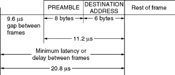
Figure 11.19: Switch Latency Includes a Built-In Delay Resulting from the Structure of the Ethernet Frame
11.3.1.17 Management
The most common method used to provide switch management involves the integration of RMON support for each switch port. This enables an SNMP console to obtain statistics from the RMON group or groups supported by each switch. Because the retrieval of statistics on a port-by-port basis can be time consuming, most switches that support RMON also create a database of statistics to facilitate their retrieval.
11.3.1.18 Mirrored Port
A mirrored port is a port that duplicates traffic on another port. For traffic analysis and intrusive testing, the ability to mirror data exiting the switch on one port to a port to which test equipment is connected can be a very valuable feature.
11.3.1.19 Module Insertion
Modular switches support two different methods of module insertion: switch power-down and hot insertion. As their names imply, a switch power-down method requires you to first deactivate the switch and literally bring it down. In comparison, the ability to perform hot insertions enables you to add modules to an operating switch without adversely affecting users.
11.3.1.20 Port Buffer Size
Switch designers incorporate buffer memory into port cards as a mechanism to compensate for the difference between the internal speed of the switch and the operating rate of an end station or segment connected to the port. Some switch designers increase the amount of buffer memory incorporated into port cards to use in conjunction with a flow control mechanism, while other switch designers can use port buffer memory as a substitute for flow control. If used only as a mechanism for speed compensation, the size of port buffers may be limited to a few thousand bytes of storage. When used in conjunction with a flow control mechanism or as a flow control mechanism, the amount of buffer memory per port may be up to 64, 128, or 256 Kbytes, perhaps even up to 1 or 2 Mbytes. Although you might expect more buffer memory to provide better results, this may not necessarily be true. For example, assume a workstation on a segment is connected to a port that has a large buffer with just enough free memory to accept one frame. When the workstation transmits a sequence of frames, only the first is able to be placed into the buffer. If the switch then initiates flow control as the contents of its port buffer is emptied, subsequent frames are barred from moving through the switch. When the switch disables flow control, it is possible that another station with data to transmit is able to gain access to the port prior to the station that sent frame one in a sequence of frames. Due to the delay in emptying the contents of a large buffer, it becomes possible that subsequent frames are sufficiently delayed as they move through a switch to a mainframe via a gateway that a time-dependent session could time-out. Thus, you should consider your network structure in conjunction with the operating rate of switch ports and the amount of buffer storage per port to determine if an extremely large amount of buffer storage could potentially result in session timeouts. Fortunately, most switch manufacturers limit port buffer memory to 128 Kbytes, which at 10 Mbps results in a maximum delay of:
or 0.10 seconds. At 100 Mbps, the maximum delay is reduced to 0.01 seconds, while at 1 Gbps the delay becomes 0.001 seconds.
11.3.1.21 Port Module Support
Although many Ethernet switches are limited to supporting only Ethernet networks, the type of networks supported can considerably differ between vendor products as well as within a specific vendor product line. Thus, you may wish to examine the support of port modules for connecting 10BASE-2, 10BASE-5, 10BASE-T, 100BASE-T LANs, and Gigabit Ethernet devices. In addition, if your organization supports different types of LANs or is considering the use of switches to form a tier structured network using a different type of high-speed backbone, you should examine port support for FDDI, full-duplex Token Ring, and ATM connectivity. Many modular Ethernet switches include the ability to add translating bridge modules, enabling support for several different types of networks through a common chassis.
11.3.1.22 Spanning Tree Support
Ethernet networks use the spanning tree algorithm to prevent loops that, if enabled, could result in the continuous replication of frames. In a bridged network, spanning tree support is accomplished by the use of bridge protocol data units (BPDUs) that enable bridges to select a root bridge and agree upon a network topology that precludes loops from occurring. Because a switch, in effect, represents a sophisticated bridge, we would want to preclude the use of multiple switches from forming a loop. For example, consider Figure 11.20, which illustrates the use of two switches to interconnect two LANs. If both switches were active, a frame from the client connected on LAN A destined to the server on LAN B would be placed back onto LAN A by Switch 1, causing a packet loop and the replication of the packet, a situation we want to avoid. By incorporating spanning tree support into each switch, they can communicate with one another to construct a topology that does not contain loops. For example, one switch in Figure 11.20 would place a port in a blocking mode while the other switch would have both ports in a forwarding mode of operation.
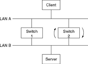
Figure 11.20: The Need for Loop Control
To obtain the ability to control the spanning tree, most switches permit a number of parameters to be altered from their management console. Those parameters include the forwarding delay, which governs the time the switch will wait prior to forwarding a packet, the aging time the switch waits for the receipt of a hello packet before initiating a topology change, the "Hello" time interval between the transmission of BPDU frames, and the path cost assigned to each port.
11.3.1.23 Switch Type
As previously discussed, a switch will either support one or multiple addresses per port. If it supports one address per port, it is a port-based switch. In comparison, if it supports multiple addresses per port, it is considered a segment-based switch even if only one end station is connected to some or all ports on the switch.
11.3.1.24 Switching Mode
Ethernet switches can be obtained to operate in a cut-through, store-and-forward, or hybrid operating mode. As previously discussed in this chapter, the hybrid mode of operation represents toggling between cut-through and store-and-forward based upon a frame error rate threshold. That is, a hybrid switch might initially be set to operate in a cut-through mode and compute the CRC for each frame on-the-fly , comparing its computed values to the CRCs appended to each frame. When a predefined frame error threshold is reached, the switch would change its operating mode to store-and-forward, enabling erroneous frames to be discarded. Some switch vendors reference a hybrid switch mode as an error-free cut-through operating mode.
11.3.1.25 Virtual LAN Support
A virtual LAN (vLAN) can be considered to represent a broadcast domain created through the association of switch ports, MAC addresses, or a network layer parameter. Thus, there are three basic types of vLAN creation methods you can evaluate when examining the functionality of an Ethernet switch. In addition, some vendors now offer a rules-based vLAN creation capability that enables users to have an almost infinite number of vLAN creation methods with the ability to go down to the bit level within a frame as a mechanism for vLAN associations.
11.3.2 Switched-Based Virtual LANs
As briefly mentioned in our review of switch features, a virtual LAN (vLAN) can be considered to represent a broadcast domain. This means that transmission generated by one station assigned to a vLAN is only received by those stations predefined by some criteria to be in the domain. Thus, to understand how vLANs operate requires us to examine how they are constructed.
11.3.2.1 Construction Basics
A vLAN is constructed by the logical grouping of two or more network nodes on a physical topology. To accomplish this logical grouping, you must use a vLAN-"aware" switching device. Those devices can include intelligent switches, which essentially perform bridging and operate at the Media Access Control (MAC) layer, or routers, which operate at the network layer, or layer 3, of the Open Systems Interconnection (ISO) Reference Model. Although a switching device is required to develop a vLAN, in actuality it is the software used by the device that provides you with a vLAN capability. That is, a vLAN represents a subnetwork or broadcast domain defined by software and not by the physical topology of a network. Instead, the physical topology of a network serves as a constraint for the software-based grouping of nodes into a logically defined network.
11.3.2.2 Implicit versus Explicit Tagging
The actual criteria used to define the logical grouping of nodes into a vLAN can be based on implicit or explicit tagging. Implicit tagging, which in effect eliminates the use of a special tagging field inserted into frames or packets, can be based on MAC address, port number of a switch used by a node, protocol, or another parameter that nodes can be logically grouped into. Because many vendors offering vLAN products use different construction techniques, interoperability between vendors may be difficult, if not impossible. In comparison, explicit tagging requires the addition of a field into a frame or packet header. This action can result in incompatibilities with certain types of vendor equipment as the extension of the length of a frame or packet beyond its maximum can result in the inability of such equipment to handle such frames or packets. Based on the preceding , the differences between implicit and explicit tagging can be considered akin to the proverbial statement "between a rock and a hard place." Although standards can be expected to resolve many interoperability problems, network managers and administrators may not have the luxury of time to wait until such standards are developed. Instead, you may wish to use existing equipment to develop vLANs to satisfy current and evolving organizational requirements.
11.3.3 Port-Grouping vLANs
As its name implies, a port-grouping vLAN represents a virtual LAN created by defining a group of ports on a switch or router to form a broadcast domain. Thus, another common name for this type of vLAN is a port-based virtual LAN.
11.3.3.1 Operation
Figure 11.21 illustrates the use of an intelligent LAN switch to create two vLANs based upon port groupings. In this example, the switch was configured to create one virtual LAN consisting of ports 0, 1, 5, and 6, while a second virtual LAN was created based upon the grouping of ports 2, 3, 4, and 7 to form a second broadcast domain.
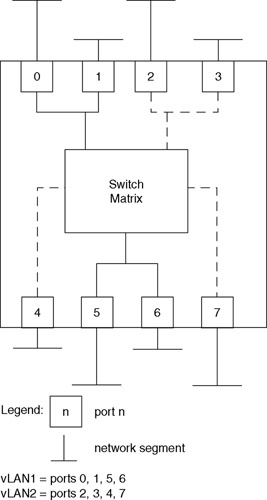
Figure 11.21: Creating Port-Grouping vLANs Using a LAN Switch
Advantages associated with the use of LAN switches for creating vLANs include the ability to use the switching capability of the switch, the ability to support multiple stations per port, and an internetworking capability. A key disadvantage associated with the use of port-based vLANs is the fact they are limited to supporting one vLAN per port. This means that moves from one vLAN to another will affect all stations connected to a particular switch port.
11.3.3.2 Supporting Inter-vLAN Communications
The use of multiple network interface cards (NICs) provides an easy-to-implement solution to obtaining an inter-vLAN communications capability when only a few vLANs must be linked. This method of inter-vLAN communications is applicable to all methods of vLAN creation; however, when a built-in routing capability is included in a LAN switch, you would probably prefer to use the routing capability rather than obtain and install additional hardware.
Figure 11.22 illustrates the use of a server with multiple NICs to provide support to two port-based vLANs. Not only does this method of multiple vLAN support require additional hardware and the use of multiple ports on a switch or wiring hub, but, in addition, the number of NICs that can be installed in a station is typically limited to two or three. Thus, the use of a large switch with hundreds of ports configured for supporting three or more vLANs may not be capable of supporting inter-vLAN communications unless a router is connected to a switch port for each vLAN on the switch.
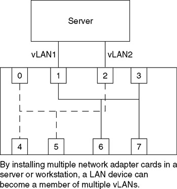
Figure 11.22: Overcoming the Port-Based Constraint Where Stations Can Join Only a Single vLAN
11.3.4 MAC-Based VLANs
Figure 11.23 illustrates the use of an 18-port switch to create two vLANs. In this example, 18 devices are shown connected to the switch via six ports, with four ports serving individual network segments. Thus, the LAN switch in this example is more accurately referenced as a segment switch with a MAC or layer 2 vLAN capability. This type of switch can range in capacity from small 8- or 16-port devices capable of supporting segments with up to 512 or 1024 total addresses, to large switches with hundreds of ports capable of supporting thousands of MAC addresses. For simplicity of illustration, we will use the six-port segment switch to denote the operation of layer 2 vLANs as well as their advantages and disadvantages.
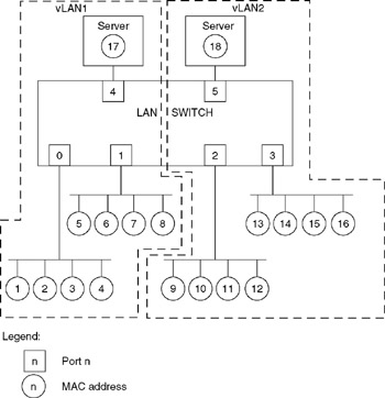
Figure 11.23: Layer 2 vLAN
In turning our attention to the vLANs shown in Figure 11.23, note that we will use the numeric or node addresses shown contained in circles as MAC addresses for simplicity of illustration. Thus, addresses 1 through 8 and 17 would be grouped into a broadcast domain representing vLAN1, while addresses 9 through 16 and 18 would be grouped into a second broadcast domain to represent vLAN2. At this point in time, you would be tempted to say "so what," as the use of MAC addresses in creating layer 2 vLANs resembles precisely the same effect as if you used a port-grouping method of vLAN creation. For example, using an intelligent hub with vLAN creation based upon port grouping would result in the same vLANs as those shown in Figure 11.23 when ports 0, 1, and 4 are assigned to one virtual LAN and ports 2, 3, and 5 to the second.
11.3.4.1 Flexibility
To indicate the greater flexibility associated with the use of equipment that supports layer 2 vLAN creation, let us assume users with network node addresses 7 and 8 were just transferred from the project associated with vLAN1 to the project associated with vLAN2. If you were using a port-grouping method of vLAN creation, you would have to physically re-cable nodes 7 and 8 to either the segment connected to port 2 or the segment connected to port 3. In comparison, when using a segment switch with a layer 2 vLAN creation capability, you would use the management port to delete addresses 7 and 8 from vLAN1 and add them to vLAN2. The actual effort required to do so might be as simple as dragging MAC addresses from one vLAN to the other when using a GUI (graphical user interface) or entering one or more commands when using a command-line management system. The top of Figure 11.24 illustrates the result of the previously mentioned node transfer. The lower portion of Figure 11.24 shows the two vLAN layer 2 tables, indicating the movement of MAC addresses 7 and 8 to vLAN2.
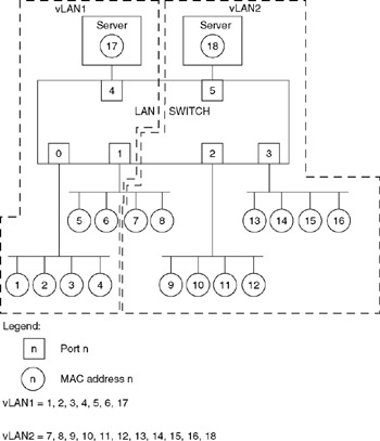
Figure 11.24: Moving Stations When Using a Layer 2 vLAN
Although the reassignment of stations 7 and 8 to vLAN2 is easily accomplished at the MAC layer, it should be noted that the "partitioning" of a segment into two vLANs can result in upper layer problems. This is because upper layer protocols, such as IP, require all stations on a segment to have the same network address. Some switches overcome this problem by dynamically altering the network address to correspond to the vLAN on which the station resides. Other switches without this capability restrict the creation of MAC-based vLANs to one device per port, in effect limiting the creation of vLANs to port-based switches.
11.3.4.2 Interswitch Communications
Similar to the port-grouping method of vLAN creation, a MAC-based vLAN is normally restricted to a single switch. However, some vendors include a management platform that enables multiple switches to support MAC addresses between closely located switches. Unfortunately, neither individual or closely located switches permit an expansion of vLANs outside the immediate area, resulting in the isolation of the virtual LANs from the remainder of the network. This deficiency can be alleviated in two ways. First, for inter-vLAN communications, you could install a second adapter card in a server and associate one MAC address with one vLAN while the second address is associated with the second virtual LAN. While this method is appropriate for a switch with two vLANs, you would require a different method to obtain interoperability when communications are required between a large number of virtual LANs. Similar to correcting the interoperability problem with the port-grouping method of vLAN creation, you would have to use routers to provide connectivity between MAC-based vLANs and the remainder of your network.
11.3.4.3 Router Restrictions
When using a router to provide connectivity between vLANs, there are several restrictions you must consider. Those restrictions typically include a requirement to use a separate switch port connection to the router for each virtual LAN and the inability to assign portions of segments to different vLANs. Concerning the former, unless the LAN switch either internally supports layer 3 routing or provides a "trunking" or "aggregation" capability that enables transmission from multiple vLANs to occur on a common port to the router, one port linking the switch to the router will be required for each vLAN. Because router and switch ports are relatively costly, internetworking of a large number of virtual LANs can become expensive. Concerning the latter, this requirement results from the fact that in a TCP/IP environment, routing occurs between segments. An example of inter-vLAN communications using a router is illustrated in Figure 11.25.
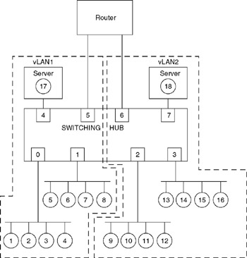
Figure 11.25: Inter-vLAN Communications Require the Use of a Router
When inter-vLAN communications are required, the layer-2 switch transmits packets to the router via a port associated with the virtual LAN workstation requiring such communications. The router is responsible for determining the routed path to provide inter-vLAN communications, forwarding the packet back to the switch via an appropriate router-to-switch interface. Upon receipt of the packet, the switch uses bridging to forward the packet to its destination port.
Returning to Figure 11.25, a workstation located in vLAN1 requiring communications with a workstation in vLAN2 would have its data transmitted by the switch on port 5 to the router. After processing the packet, the router would return the packet to the switch, with the packet entering the switch on port 6. Thereafter, the switch would use bridging to broadcast the packet to ports 2, 3, and 7, where it would be recognized by a destination node in vLAN2 and copied into an appropriate network interface card.
11.3.5 Layer 3-Based vLANs
A layer 3 based vLAN is constructed using information contained in the network layer header of packets. As such, this precludes the use of LAN switches that operate at the data-link layer from being capable of forming layer 3 vLANs. Thus, layer 3 vLAN creation is restricted to routers and LAN switches that provide a layer 3 routing capability.
Through the use of layer 3 operating switches and routers, there are a variety of methods that can be used to create layer 3 vLANs. Some of the more common methods supported resemble the criteria by which routers operate, such as IPX network numbers and IP subnets, AppleTalk domains, and layer 3 protocols.
The actual creation options associated with a layer 3 vLAN can vary considerably based upon the capability of the LAN switch or router used to form the virtual LAN. For example, some hardware products permit a subnet to be formed across a number of ports and may even provide the capability to allow more than one subnet to be associated with a network segment connected to the port of a LAN switch. In comparison, other LAN switches may be limited to creating vLANs based upon different layer 3 protocols.
11.3.5.1 Subnet-Based vLANs
Figure 11.26 illustrates the use of a layer 3 LAN switch to create two virtual LANs based upon IP network addresses. In examining the vLANs created through the use of the LAN switch, note that the first virtual LAN is associated with the subnet 198.78.55, which represents a Class C IP address, while the second vLAN is associated with the subnet 198.78.42, which represents a second Class C IP address. Also note that because it is assumed that the LAN switch supports the assignment of more than one subnet per port, port 1 on the switch consists of stations assigned to either subnet. While some LAN switches support this subnetting capability, it is also important to note that other switches do not. Thus, a LAN switch that does not support multiple subnets per port would require stations to be re-cabled to other ports if it was desired to associate them to a different virtual LAN.
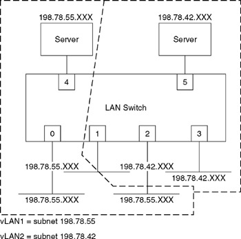
Figure 11.26: vLAN Creation Based on IP Subnets
11.3.5.2 Protocol-Based vLANs
In addition to forming virtual LANs based on a network address, the use of the layer 3 transmission protocol as a method for vLAN creation provides a mechanism that enables vLAN formation to be based on the layer 3 protocol. Using this method of vLAN creation, it becomes relatively easy for stations to belong to multiple vLANs. To illustrate this concept, consider Figure 11.27, which illustrates the creation of two vLANs based on their layer 3 transmission protocol. In examining the stations shown in Figure 11.27, note that the circles with the uppercase I represent those stations configured for membership in the vLAN based upon the use of the IP protocol, while those stations represented by circles containing the uppercase X represent stations configured for membership in the vLAN that uses the IPX protocol as its membership criteria. Similarly, stations represented by circles containing the characters I/X represent stations operating dual protocol stacks that enable such stations to become members of both vLANs.
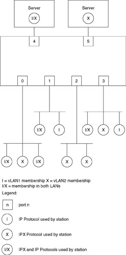
Figure 11.27: vLAN Creation Based on Protocol
Two servers are shown at the top of the LAN switch illustrated in Figure 11.27. One server is shown operating dual IPX/IP stacks, which results in the server belonging to both vLANs. In comparison, the server on the upper right of the switch is configured to support IPX and could represent a NetWare file server restricted to membership in the vLAN associated with the IPX protocol.
11.3.5.3 Rule-Based vLANs
A recent addition to vLAN creation methods is based on the ability of LAN switches to look inside packets and use predefined fields, portions of fields, and even individual bit settings as a mechanism for the creation of a virtual LAN.
11.3.5.4 Capabilities
The ability to create virtual LANs via a rule-based methodology provides, no pun intended, a virtually unlimited virtual LAN creation capability. To illustrate a small number of the almost unlimited methods of vLAN creation, consider Table 11.3, which lists eight examples of rule-based vLAN creation methods. In examining the entries in Table 11.3, note that in addition to creating vLANs via the inclusion of specific field values within a packet, such as all IPX users with a specific network address, it is also possible to create vLANs using the exclusion of certain packet field values. The latter capability is illustrated by the next to last example in Table 11.3, which forms a vLAN consisting of all IPX traffic with a specific network address but excludes a specific node address.
|
11.3.5.5 Multicast Support
One rule-based vLAN creation example that deserves a degree of explanation to understand its capability is the last entry in Table 11.3. Although you might be tempted to think that the assignment of a single IP address to a vLAN represents a typographical mistake, in actuality it represents the ability to enable network stations to dynamically join an IP multicast group without adversely affecting the bandwidth available to other network users assigned to the same subnet, but located on different segments attached to a LAN switch. To understand why this occurs, let us digress and discuss the concept associated with IP multicast operations.
IP multicast references a set of specifications that allows an IP host to transmit one packet to multiple destinations. This one-to-many transmission method is accomplished using Class D IP addresses (224.0.0.0 to 239.255.255.255), which are mapped directly to data-link layer 2 multicast addresses. Through the use of IP multicasting, a term used to reference the use of Class D addresses, the need for an IP host to transmit multiple packets to multiple destinations is eliminated. This, in turn , permits more efficient use of backbone network bandwidth; however, the arrival of IP Class D addressed packets at a network destination, such as a router connected to an internal corporate network, can result in a bandwidth problem. This is because multicast transmission is commonly used for audio and/or video distribution of educational information, videoconferencing, news feeds, and financial reports , such as delivering stock prices. Due to the amount of traffic associated with multicast transmission, it could adversely affect multiple subnets linked together by a LAN switch that uses subnets for vLAN creation. By providing a "registration" capability that allows an individual LAN user to become a single-user vLAN associated with a Class D address, Class D packets can be routed to a specific segment even when several segments have the same subnet. Thus, this limits the effect of multicast transmission to a single segment.
11.3.6 Upper Layer Switching
In concluding this chapter, we briefly turn our attention to upper layer switches, a term used by this author to collectively denote switching performed at ISO Open System Interconnection (OSI) Reference Model layers above the data-link layer. Beginning in the latter portion of 1996, vendors introduced switching products that operate at layer 3, the network layer, and even layer 4, the transport layer. By 2002, vendors had extended switching capability to the application layer, layer 7 in the ISO Reference Model.
Switches operating above layer 2 are based on the need to provide network users with a higher degree of functionality. Although we can truthfully state that switches operating above layer 2 look deeper into the frame to examine higher layer packet data encapsulated in LAN frames, that is a simplistic view of such switches. To obtain a better appreciation for the operation and utilization of upper layer switches, let us first examine the rationale for the development of such switches.
11.3.6.1 Rationale
A layer 2 switch operates using MAC addresses. In doing so, it views all interconnected networks as flat, requiring flooding to occur when the destination address in a frame is unknown. Using a flat network view, the higher capacity of layer 2 LAN switches over traditional shared media hubs begins to be negated due to redundant traffic being carried over switch-based networks as well as broadcast storms occurring on such networks. As previously discussed in this chapter during our examination of virtual LANs, the introduction of vLAN capability to layer 2 LAN switches enabled users to partition a switch into broadcast domains, which alleviates some of the effect of broadcasts interfering with data transfer. However, unless you create a large number of vLANs, which introduces inter-vLAN communications problems, you will continue to have broadcast problems.
Another limitation of layer 2 switches is the fact that they are based on layer 2 addresses. This means that they are not capable of recognizing the structure of a hierarchical network nor taking advantage of that network structure.
Because layer 2 LAN switches operate considerably faster than routers that operate at the network layer, such switches achieve a high degree of penetration in isolated islands of corporate LANs. However, routers are still required to move packets between geographically separated networks or to collapse the layer 2 switch infrastructure using the router as a backbone device. An example of the latter is shown in Figure 11.28, where a router is used to link two switches together as well as provide a WAN connection to a distant network location.
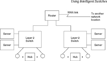
Figure 11.28: Using a Router to Interconnect Switches
One of the problems associated with using routers to collapse switch-based networks, provide inter-vLAN communications, and perform other functions is the fact that they are relatively slow in comparison to the operation of layer 2 switches. Conventional routers are software-based devices that use microprocessors to perform such traditional functions as looking up next-hop route information, modifying packet headers, and forwarding packets out an appropriate router port. As it operates at layer 3, a conventional router must update the time-to-live (TTL) field in IP packets, recalculate the frame check sequence (FCS), and perform other network- related functions that limit the number of packets per second that can be processed . Layer 2 switches commonly perform most tasks in hardware, using application specific integrated circuits (ASICs) to achieve frame processing rates in the millions of frames per second. In comparison, conventional routers may be hard-pressed to operate above 5000 packets per second as they perform the previously described operations via software.
The performance problems associated with routers used to interconnect layer 2 switches as well as the need to developing faster processing capabilities for internetworking applications, such as the use of routers to transmit packets on the Internet, resulted in the incorporation of several techniques to enhance the packet processing capability of routers. Those techniques include the use of ASICs and special headers appended to packets to identify traffic flows and facilitate their routing. The latter technique is more commonly referred to as tag switching and standardized as Multi-protocol Label Switching (MPLS). Now that we have an overview of the rationale for the development of higher layer switching, let us turn our attention to the methods used to obtain this capability.
11.3.6.2 Layer 3 Switching
When we discuss layer 3 switching, we are really talking about a wide range of products that operate at the network layer. Some products are LAN switches with a built-in simplistic routing capability that enables the switch to look into each frame to the network layer and make switching decisions based upon the type of protocol network address (as previously discussed during our examination of virtual LANs). Other layer 3 switching products are actually designed to forward packets at extremely high data rates beyond the capabilities of conventional routers. As such, they are manufactured for providing transmission over a wide area network in comparison to layer 3 LAN switches that provide a vLAN creation capability on a local area network. To obtain the high-speed packet processing capability, the second type of router either is designed to use ASICs for processing each packet or creates flows to facilitate the movement of packets. Thus, we can further categorize layer 3 switching by the manner by which packets are processed: packet by packet or flow based.
11.3.6.3 Packet-by-Packet Routing
When layer 3 switching uses a packet-by-packet routing method, the router, or perhaps a better term to use is the switch/router, examines each packet via hardware and forwards it to its destination using standardized routing protocols. Through the use of ASICs to perform a majority of traditional router functions as well as the replacement of a bus-based architecture by either a shared-memory or crossbar architecture, switch/router packet processing performance is significantly enhanced.
A key advantage of the switch/router that operates on a packet-by-packet basis is its compatibility with other routers in the network. Such switch/ routers do not need to recognize special packet headers that are employed by the second type of layer 3 switch, one that uses flow-based routing.
11.3.6.4 Flow-Based Routing
Layer 3 flow-based switching was developed by Ipsilon Networks in 1996 and was shortly followed by other vendors that introduced their own methods for using network addresses for high-speed switch/router products. Here, the term "flow" represents a conversation between two end stations through a network. Flow-based switching requires tags to be appended to packets to expedite their delivery and was standardized as MPLS.
In flow-based routing, an initial packet or group of packets is identified to determine if they are flowing to a common destination and if the packet is part of a larger sequence of packets, with the latter occurring by examining packet sequence numbers and the window size negotiated during a TCP/IP session. During this initial flow learning process, the first or first few packets are routed. Once a flow is identified, a mechanism is used to inform all intermediate devices between flow points of the flow so they can use switching instead of routing.
One of the most popular methods used to identify a flow is to prefix a tag to the packet. This technique, which is referred to as tag switching, was initially used by Cisco Systems prior to the standardization of MPLS.
Figure 11.29 illustrates an example of the partial construction of router flow tables assuming the use of packet tagging. In this example, assume a flow from station 1 on LAN A to station 5 on LAN 3 was identified and assigned a tag value of 6. Router 1 would prefix each packet inbound from port 2 that meets the flow criteria with tag number 6 and by examining its flow table switch packets with tag 6 out port 3. At router 2, packets inbound with a tag value of 6 would be switched out of port 3. In tag switching, each router between flow points only has to examine the tag to determine how to switch the incoming packet, significantly enhancing the packet per second processing rate of the switch/router. However, each router between flow points must be capable of supporting tag switching or another type of layer 3 forwarding based upon the type of forwarding used by the network.
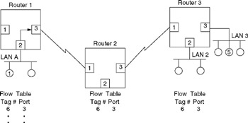
Figure 11.29: Flow-Based Routing Using Packet Tagging Assuming Flow from Station 1 on LAN A to Station 5 on LAN 3 Is Identified by Tag Number 6
Although flow-based routing can considerably enhance the packet processing rate of switch/routers, this method of routing originally represented proprietary solutions that did not provide interoperability between different vendor products. This situation changed with the standardization of MPLS.
A current limitation of flow-based routing is the fact that you cannot use such network applications as traceroute to determine the route to a destination because the use of tags or labels results in a proprietary route development mechanism through the network. However, if you need an extremely high packet processing capability, a flow-based layer 3 switching technique may provide the solution to your organization's processing requirements.
11.3.6.5 Layer 4 Switching
A layer 4 switch looks further into each packet, examining layer 4 information such as the contents of the TCP or the UDP header. Once this information is obtained, the layer 4 switch becomes capable of making decisions concerning the routing of traffic based upon the type of application being carried by the packet. Because a sequence of packets carrying a particular application results in a session of activity, another term for a layer 4 switch is a "session switch."
By examining the start of a transmission session via noting a SYN packet or a TCP start, the switch can be used to provide a number of functions that can be difficult, if not impossible, for layer 2 and layer 3 switches to perform. For example, by examining the TCP or UDP port numbers, a layer 4 switch can bind sessions to specific IP addresses based on the use of predefined criteria, such as the flow of traffic to two or more servers. To illustrate this, consider the use of the layer 4 LAN switch that is shown in Figure 11.30. In this example, the layer 4 switch can function as a load balancer or application distributor.
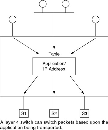
Figure 11.30: Using a Layer 4 Switch
In the example illustrated in Figure 11.30, the layer 4 switch could function as a virtual IP (VIP) front end to the servers connected to the switch. Here, a VIP address would be configured for each server or group of servers that supports a single or a common application. Once the switch determines the appropriate server to satisfy a session, it binds the session to a specific IP address and substitutes the server's real IP address for the virtual IP address. Once the preceding is accomplished, the layer 4 switch forwards the connection request and subsequent packets, remapping the addresses of the packets until a session termination or FIN packets are encountered .
In general, layer 4 switches are slower than layer 2 switches because they must look further into the packet, requiring additional processing time. In addition, layer 4 switches are primarily designed for intranet applications. Thus, while layer 4 switches can provide a relatively high-speed packet processing capability, their layer 3 operations may be limited, with many routing protocols not supported by the switch.
Although the use of layer 4 switching is primarily to note application sessions and route those sessions to an appropriate port, it should be noted that when functioning as a traffic balancer, the switch represents a much more capable product than a hardware-based load balancer. Concerning the latter, a load balancer is typically a two to four LAN, one WAN port device that simply routes incoming Web traffic requests to mirrored servers. In comparison, a layer 4 switch can route all types of traffic and can range in size from a few ports to hundreds of ports.
11.3.6.6 Application Layer Switching
An application layer switch would appear to operate at layer 7 of the ISO Reference Model. While this assumption is correct for some protocol stacks, because an application in the TCP/IP protocol suite is identified by port number, application layer switching can occur at layer 4. Thus, in a TCP/IP environment, application layer switching occurs through the use of a layer 4 switch.
EAN: 2147483647
Pages: 111