4.1 Waiting Line Analysis

Queuing theory, the formal term for waiting line analysis, can be traced to the work of A.K. Erlang, a Danish mathematician . His pioneering work spanned several areas of mathematics, including the dimensioning or sizing of trunk lines to accommodate long-distance calls between telephone company exchanges. Readers are referred Chapter 5 for specific information concerning the application of Erlang's work conducted during the 1920s to the sizing of ports on modern LAN access devices. In this chapter we bypass Erlang's sizing work to concentrate on the analysis of waiting lines.

4.1.1 Basic Components

Figure 4.1 illustrates the basic components of a simple waiting line system. The input process can be considered the arrival of people, objects, or frames of data. The service facility performs some predefined operation on arrivals, such as collecting tolls from passengers in cars arriving at a toll booth , or converting a LAN frame into an SDLC or HDLC frame by a remote bridge or router for transmission over a WAN transmission facility. If the arrival rate temporarily exceeds the service rate of the service facility, a waiting line known as a queue will form. If a waiting line never exists, this fact implies that the server is idle or an excessive service capacity exists.

Figure 4.1: Basic Components of a Simple Waiting Line System

The waiting line system illustrated in Figure 4.1 is more formally known as a single-channel, single-phase waiting line system. The term "single channel" refers to the fact that there is one waiting line, while the term "single phase" refers to the fact that the process performed by the service facility occurs once at one location. One toll booth on a highway or a single-port remote bridge or router connected to a local area network and a wide area network are two examples of single-channel, single-phase waiting line systems.

Figure 4.2 illustrates three additional types of waiting line systems. Here, the term "multiple channel" refers to the fact that arrivals are serviced by more than one service facility and results in multiple paths or channels to those service facilities. The term "multiple phas e " references the fact that arriving entities are processed by multiple service facilities.

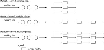
Figure 4.2: Other Types of Waiting Line Systems

One example of a multiple-phase service facility would be a toll road in which drivers of automobiles are serviced by several series of toll booths. Any reader who drove on the Petersburg “Richmond, Virginia, turnpike during the 1980s is probably well aware of the large number of 25 toll booths you seemed to have encountered every few miles. Another example of a multiple phase would be the routing of data through a series of bridges and routers. Because the computations associated with multiple phase systems can become quite complex and we can analyze most networks on a point-to-point basis as a single phase system, we will primarily restrict our examination of queuing models to single phase systems in this chapter.

4.1.2 Assumptions

Queuing theory is similar to many other types of mathematical theory in that it is based on a series of assumptions. Those assumptions primarily focus on the distribution of arrivals and the time required to service each arrival.

If the arrival rate is stochastic (i.e., it varies in some random fashion over time), we need to further classify it through the use of a probability distribution because arrivals can appear either singularly or in batches. A second method of categorizing the arrival rate occurs when arrivals occur at a fixed rate, with a fixed time between successive arrivals. This second type of arrival is referred to as deterministic. The Greek letter lambda ( » ) is normally used to denote the arrival rate.

The time required to service arrivals is referred to as the service rate and can also be stochastic or deterministic. The Greek letter ¼ is normally used to represent the service rate.

Both the distribution of arrivals and the time to service them are normally represented as random variables . The most common distribution used to represent arrivals is the Poisson distribution, where:

where:

P(n)	= probability of n arrivals
»	= mean arrival rate
e	= 2.71828
n!	= n factorial n(n ˆ’ 1) 32*1

One of the more interesting features of the Poisson process concerns the relationship between the arrival rate and the time between arrivals. If the number of arrivals per unit time is Poisson distributed with a mean of » , then the time between arrivals is distributed as a negative exponential probability distribution with a mean of 1/ » . For example, if the mean arrival rate per 10-minute period is 3, then the mean time between arrivals is 10/3, or 3.3 minutes.

4.1.3 Queuing Classifications

The previously described relationship between Poisson arrival time and a negative exponential service rate is referred to as an M/M/1 queuing system. A queuing system format was developed by Kendall to provide a mechanism for classifying different types of queuing systems. The general format of Kendall's classification scheme is:

where:

A specifies the inter-arrival time distribution
B specifies the service time distribution
X specifies the number of service channels
Y specifies the system capacity
Z specifies the queue discipline

The letter M used to describe a queuing system that has a Poisson arrival time, and a negative exponential service time denotes that the inter-arrival time and service time distributions are memory-less. When the system capacity and queue are considered to be infinite, the designators Y and Z are omitted. As we will note later in this chapter, as the level of utilization of a system increases , the difference between infinite and finite system capacity and queue length decreases. Because we often are primarily interested in determining the effect on a system under a high level of utilization, both infinite and finite models can provide satisfactory information.

4.1.4 Network Applications

Through the use of queuing theory or waiting time analysis, we can examine the effect of different WAN circuit operating rates. That is, we can examine the ability of remote bridges and routers to transfer data between LANs, and the effect of different levels of buffer memory on their ability to transfer data. In doing so we can obtain answers to such critical questions as: What is the average delay associated with the use of a remote bridge or router? What is the effect on those delays by increasing the operating rate of the WAN circuit? When does an increase in the wide area network circuit's operating rate result in an insignificant improvement in bridge or router performance? How much buffer memory should a remote bridge or router contain to avoid losing frames? To illustrate the application and value of queuing theory to network problems, let us look at an example of its use.

Let us assume you are planning to interconnect two geographically dispersed LANs through the use of a pair of routers or remote bridges as illustrated in Figure 4.3. In this example, a Token Ring network at one location will be connected to an Ethernet LAN at another location. Most routers and remote bridges support both RS-232 and V.35 interfaces, permitting the router or bridge to be connected to modems or higher-speed data service units (DSUs) that are used with digital transmission facilities. This opens a Pandora's box concerning the type of circuit to use to connect a pair of remote bridges, analog or digital, and the operating rate of the circuit. Fortunately, we can use queuing theory to determine an optimum line operating rate to interconnect the two LANs illustrated in Figure 4.3.

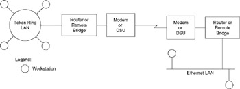
Figure 4.3: Connecting Two Geographically Separated LANs via a Pair of Routers or Remote Bridges

4.1.5 Deciding on a Queuing Model

In applying queuing theory to the network configuration illustrated in Figure 4.3, you would be correct in stating that it resembles a single-channel, multiple-phase waiting line system similar to the second example shown in Figure 4.2. However, prior to deciding on a queuing model to use, let us consider the delays associated with each phase of the network shown in Figure 4.3.

If data is routed from the Token Ring network to the Ethernet network, the primary delay occurs when a frame attempts to gain access to the router or bridge connected to the Token Ring LAN and use its encapsulation services to be placed onto the WAN. If the memory of the router or bridge is not full, the frame is placed into memory at the LAN's operating rate. After a delay based on the number of frames preceding that frame just placed in memory, it is transmitted bit by bit at the WAN operating rate, which is typically an order of magnitude lower than the LAN operating rate. If the memory of the router or bridge is full, the frame is discarded and the workstation that originated the frame must then retransmit it, further adding to the delay in the frame reaching its destination. At the Ethernet site, the frame is received on a bit-by-bit basis and the primary delay encountered is the time required to buffer the frame for placement on the Ethernet LAN.

Because multiple frames result in one following another, there is a degree of overlap between receiving frame n+1 and placing received frame n onto the network. In addition, because the WAN operating rate is but a fraction of the LAN operating rate, the delay associated with the destination router or bridge becomes primarily one of latency and is negligible with respect to the bridge at the transmit side of the interconnected network. Due to this we can simplify our computations by assuming that the second phase of the single-channel, multiple-phase model does not exist, thus reducing the network to a single-channel, single-phase model. Similarly, data flowing from the Ethernet to the Token Ring network has its primary delay attributable to the local router or bridge connected to the Ethernet network. Thus, dataflow in either direction can be analyzed using a single-channel, single-phase queuing model.

4.1.6 Applying Queuing Theory

Let us assume that based upon prior knowledge obtained from monitoring the transmission between locally interconnected LANs, you determined that approximately 10,000 frames per day can be expected to flow from one network to the other network. Let us also assume that the average length of each frame was determined to be 1250 bytes.

Based on the assumption that 10,000 frames will flow between each LAN, we must convert that frame rate into an arrival rate. In doing so let us further assume that each network is only active eight hours per day and both networks are in the same time zone. Thus, a transaction rate of 10,000 frames per eight- hour day is equivalent to an average arrival rate of 10,000/(8 * 60 * 60), or 0.347222 frames per second. In queuing theory, this average arrival rate (AR) is the average rate at which frames arrive at the service facility for forwarding across the WAN communications circuit.

Previously we said that through monitoring it was determined that the average frame length was 1250 bytes. Because a LAN frame must be converted into a WAN frame or packet for transmission over a WAN transmission facility, the resulting frame or packet will usually result in the addition of header and trailer information required by the protocol used to carry the LAN frame. Thus, the actual length of the WAN frame or packet will exceed the length of the LAN frame. For computational purposes, let us assume that 25 bytes are added to each LAN frame, resulting in the average transmission of 1275 bytes per frame.

Because the computation of an expected service time requires an operating rate, let us first assume that the WAN communications circuit illustrated in Figure 4.3 operates at 9600 bps. Then, the time required to transmit one 1275-byte frame or packet becomes 1275 bytes/frame * 8 bits/byte/9600 bps, or 1.0625 seconds. This time is more formally known as the expected service time and it represents the time required to transmit a frame whose average length is 1250 bytes on the LAN and 1275 bytes when converted for transmission over the WAN transmission facility. Given that the expected service time is 1.0625 seconds, we can easily compute the mean service rate (MSR). That rate is the rate at which frames entering the router or remote bridge destined for the other LAN are serviced and it is 1/1.0625, or 0.9411765 frames per second.

So far, we have computed two key queuing theory variables: the arrival rate and the mean service rate. Note that the service rate computation depended on the initial selection of a WAN circuit operating rate, which was initially selected as 9600 bps.

Figure 4.4 illustrates the results of our initial set of computations for one portion of our interconnected LANs. Because we assumed that 10,000 frames per eight-hour day flow in each direction, we can simply analyze one half of the interconnected network. This simplification is facilitated by the fact that we are also assuming that the average frame size flowing in each direction is the same or near equivalent. If this is not true, such as for internetwork communications restricted to network users on one LAN accessing a server on another network resulting in relatively short queries in one direction followed by long frames carrying responses to those queries, then our assumption would fall by the wayside. In this type of situation, you would analyze the traffic flow in each direction and select a line operating rate that meets your requirements for serving the worst-case transmission direction in terms of frame rate and frame size. However, if the traffic flow is even or near even in terms of frame rate and frame size , you can restrict your analysis to one direction. This is because full-duplex communications circuits operate at the same data rate in each direction; once you determine the required operating rate in one direction you have also determined the operating rate of the circuit.

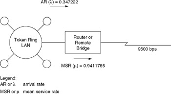
Figure 4.4: Initial Computational Results

4.1.7 Queuing Theory Designators

In examining Figure 4.4, note that queuing theory designators are indicated in parenthesis. Thus, in a queuing theory book, the average arrival rate of 0.347222 transactions or frames per second would be indicated by the expression » = 0.347222. Similarly, the mean service rate in queuing theory books is designated by the symbol ¼ .

Although the mean service rate exceeds the average arrival rate, upon occasion the arrival rate will result in a burst of data that exceeds the capacity of the router or bridge to service frames. When this situation occurs, queues are created as the router or bridge accepts frames and places those frames it cannot immediately transmit into buffers or temporary storage areas. Through the use of queuing theory, we can examine the expected time for frames to flow through the router or bridge and adjust the circuit operating rate accordingly . In addition, we can use queuing theory to determine the amount of buffer memory a remote bridge or router should have to minimize the potential for the loss of frames to a specific probability.

As previously discussed, the use of remote bridges or routers can be considered to represent a single-channel, single-phase queuing model. For this model we will assume arrivals follow a Poisson distribution and a negative exponential distribution is associated with the service rate. In addition to the preceding, we will also make the following assumptions:

There is an infinite calling population.
There is an infinite queue.
Queuing is on a first-come, first-serve basis.
Over a prolonged period of time, the service rate exceeds the arrival rate ( ¼ > » ).

The use of the preceding assumptions results in the notation M/M/1 being used to classify this queuing system. Based on the preceding, the utilization of the service facility (p) is obtained by dividing the average arrival rate by the mean service rate. That is,

Thus, the use of a circuit operating at 9600 bps results in an average utilization level of approximately 37 percent. Readers should note that in queuing theory texts , the preceding equation will be replaced by p = » / ¼ , where » is the symbol used for the average arrival rate, while ¼ is the symbol used for the mean service rate.

Because the utilization level of the service facility (router or remote bridge) is AR/MSR, the probability that there are no frames in the bridge, P , becomes:

For the remote bridge connected to a 9600-bps circuit, we then obtain:

Thus, 63 percent of the time there will be no frames in the bridge's buffers awaiting transmission to the distant network.

4.1.8 Frame Determination

For a single-channel, single-phase system, the mean number of units expected to be in the system is equivalent to the average arrival rate divided by the difference between the mean service rate and the arrival rate. In queuing theory, the mean or expected number of units in a system is normally designated by the letter L. Thus,

Returning to our networking example, we can determine the mean or expected number of frames that will be in the system, including frames residing in the device's buffer area or flowing down the WAN transmission facility as follows :

Thus, on the average, we can expect approximately six tenths of a frame to reside in the device's buffer and on the transmission line.

If we multiply the utilization of the service facility by the expected number of units in a system, we obtain the mean number of units in the queue or, in common English, the queue length. The queue length is denoted by Lq and thus becomes:

Again, returning to our network example, we obtain:

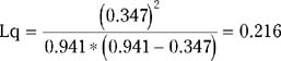
Based on the preceding, we can expect, on average, 0.216 frames to be queued in the bridge or router for transmission when the operating rate of the WAN is 9600 bps and 10,000 frames per eight-hour day require remote bridging or routing to the opposite destination. Because we previously determined that there were 0.585 frames in the system, this means that the difference, (0.585 ˆ’ 0.216) or 0.369 frames, is flowing on the transmission line at any particular point in time.

We can visualize the locations where frames are temporarily stored by examining Figure 4.5, which illustrates the relationship between L, Lq, and L ˆ’ Lq. Here, Lq corresponds to the buffer memory of the device while L corresponds to the system consisting of the bridge or router and the transmission line. Thus, L -Lq then corresponds to the frames or portion of a frame flowing on the transmission line.

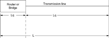
Figure 4.5: Temporary Frame Storage Relationship

The preceding information also provides us with data concerning the average expected utilization of the WAN transmission facility. Because the frame length is 1275 bytes and 0.369 frames can be expected to be flowing on the circuit at any point in time, this means the line can be expected to hold 1275 bytes/frame * 0.369 frames, or 470.5 bytes. This is equivalent to 3764 bits on a line planned to operate at 9600 bps, or a circuit utilization level of approximately 39 percent.

4.1.9 Time Computations

In addition to computing information concerning the expected number of frames in queues and in the system, queuing theory provides us with the tools to determine the mean time in the system and the mean waiting time. In queuing theory, the mean waiting time is designated by the variable W, while the mean waiting time in the queue is designated by the variable Wq.

The mean time in the system, W, is:

For our bridged network example, the mean time a frame can be expected to reside in the system can be computed as follows:

By itself, this tells us that we can expect an average response time of approximately 1.7 seconds for frames that must be bridged or routed from one LAN to the other if our WAN transmission facility operates at 9600 bps. Whether this is good or bad depends on how you view a 1.7 second delay.

The next queuing item we will focus our attention on is the waiting time associated with a frame being queued. That time, Wq, is equivalent to the waiting time in the system multiplied by the utilization of the service facility. That is,

In terms of queuing theory, Wq then becomes:

Similar to the manner by which frame storage relationships were shown with respect to the bridge and transmission line, we can illustrate the relationship of waiting times. Figure 4.6 illustrates the relationship between W, Wq, and W ˆ’ Wq with respect to the bridge and transmission line. Here, Wq corresponds to the waiting time for a frame to pass through the bridge or router, while W is the total frame waiting time to include the transit time through the device and across the transmission line. Thus, W ˆ’ Wq corresponds to the time required for a frame to transit the transmission line.

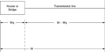
Figure 4.6: Waiting Time Relationship

Once again, let us return to our bridged network example. In doing so, we obtain:

Note that we previously determined that a frame can be expected to reside for 1.68 seconds in our communications system, including queue waiting time and transmission time. Because we computed the queue waiting time as 0.621 seconds, the difference between the two, 1.68 ˆ’ 0.621, or approximately 1.06 seconds, is the time required to transmit a frame over the 9600-bps WAN transmission facility.

Two of the more interesting relationships we should note are the variance of Lq and Wq as a function of utilization. As previously noted,

Because utilization (p) is the ratio of » / ¼ , it is difficult to vary p and compute Lq and Wq. Instead, we can fix the arrival rate and vary the service rate to change the level of utilization. Doing so also enables us to compute the length of the queue (Lq) and the waiting time in the queue (Wq).

Figure 4.7 illustrates the display of a Microsoft Excel spreadsheet developed to compute Lq and Wq based upon the level of utilization for an M/M/1 queuing system. Note that by fixing the arrival rate at unity, Lq and Wq are equal. Also note that from both the graph and tabular data presented in Figure 4.7, as the level of utilization increases beyond 70 percent, the length of the queue as well as the waiting time in the queue begin to significantly increase. In fact, this example illustrates why an increase in the level of utilization beyond 70 percent can result in significant communications problems due to a queuing system buildup and expansion in waiting time. As we will note later in this chapter, we can compensate for the buildup in system utilization by adding a faster communications channel, in effect increasing the service rate, which lowers the level of utilization. Readers are referred to the file QLENUTIL in the directory Excel at the previously noted Web URL address, which contains the spreadsheet shown in Figure 4.7. You can alter the parameters in the spreadsheet to examine the effect on Lq and Wq based upon other arrival rates and service rates.

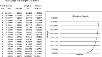
Figure 4.7: Queue Length and Waiting Time versus Utilization

4.1.10 Frames in the System

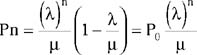
The last queuing item we focus attention on in applying the M/M/1 model is determining the number of frames in the system. As previously noted, the utilization of the system is » / ¼ . The probability of no units in an M/M/1 system is then 1 ˆ’ » / ¼ , which we defined as P . Thus, the probability that there are n units in the system becomes:

We can also determine the probability there are k or more units in the system as follows:

Because P = 1 ˆ’ P and P = » / ¼ , we can rewrite P _n>k as follows:

Later in this chapter we will examine the effect of changes in the utilization level of a queuing system upon the probability of a specific number of frames in the system.