4.2 Determining an Optimum Line Operating Rate

4.2 Determining an Optimum Line Operating Rate

Although we could recompute each of the previously computed variables based on different line operating rates, we can just as easily write a program to perform such tedious operations. Thus, let us do so.

4.2.1 Program QUEUE.BAS

Table 4.1 lists the statements of a BASIC language program appropriately named QUEUE.BAS. The execution of this program is shown in Table 4.2, which displays the values for eight queuing theory parameters based upon line speeds ranging from 4800 bps to 1.536 Mbps. The latter line speed represents the effective operating rate of a T1 circuit, because 8000 bps of the 1.544-Mbps operating rate of that circuit is used for framing and is not available for the actual transmission of data.

 REM PROGRAM QUEUE.BAS CLS PRINT "Queuing Analysis Program - Single-Phase, Single-Channel Model" REM AR=arrival rate REM MSR=mean service rate REM L=mean (expected) number of frames in system REM Lq=mean number of frames in queue REM W=mean time (s) in system REM Wq=mean waiting time (s) REM EST= expected service time INPUT "Enter transactions/day"; transactions INPUT "Enter average frame size in bytes"; avgframe PRINT hrsperday = 8 AR = transactions/(8 * 60 * 60) DATA 9600,19200,56000,64000,128000,256000,384000,768000,1536000,1984000 FOR i = 1 TO 10 READ linespeed(i) est(i) = avgframe * 8/linespeed(i) msr(i) = 1/est(i) utilization(i) = AR/msr(i) prob0(i) = 1 - (AR/msr(i)) L(i) = AR/(msr(i) - AR) Lq(i) = AR ^ 2/(msr(i) * (msr(i) - AR)) W(i) = 1/(msr(i) - AR) Wq(i) = AR/(msr(i) * (msr(i) - AR)) NEXT i PRINT "Line Speed EST   MSR     Po       p       L       Lq W Wq" FOR i = 1 TO 10 PRINT USING " #######  #.#### ###.## "; linespeed(i); est(i); msr(i); PRINT USING " #.#####.#####"; prob0(i); utilization(i); PRINT USING "  #.#####  #.#####  #.#####   #.#####"; L(i); Lq(i); W(i); Wq(i) NEXT i PRINT PRINT "where:" PRINT PRINT " EST= expected service time MSR = mean service rate" PRINT " Po=probability of zero frames in the system p = utilization" PRINT " L= mean number of frames in system Lq = mean number in queue" PRINT " W= mean waiting time in system Wq = mean waiting time in queue" 

 Line Speed EST   MSR     P   p       L       Lq      W       Wq    4800 2.1250   0.47 0.26215 0.73785 2.81457 2.07672 8.10596 5.98096    9600 1.0625   0.94 0.63108 0.36892 0.58459 0.21567 1.68363 0.62113   19200 0.5313   1.88 0.81554 0.18446 0.22618 0.04172 0.65141 0.12016   56000 0.1821   5.49 0.93676 0.06324 0.06751 0.00427 0.19444 0.01230   64000 0.1594   6.27 0.94466 0.05534 0.05858 0.00324 0.16871 0.00934  128000 0.0797  12.55 0.97233 0.02767 0.02846 0.00079 0.08196 0.00227  256000 0.0398  25.10 0.98617 0.01383 0.01403 0.00019 0.04040 0.00056  384000 0.0266  37.65 0.99078 0.00922 0.00931 0.00009 0.02681 0.00025  768000 0.0133  75.29 0.99539 0.00461 0.00463 0.00002 0.01334 0.00006 1536000 0.0066 150.59 0.99769 0.00231 0.00231 0.00001 0.00666 0.00002 where: EST = expected service time; MSR = mean service rate; P   = probability of zero frames in the system; p = utilization; L = mean number of frames in system; Lq = mean number in queue; W = mean waiting time in system; Wq = mean waiting time in queue. 

4.2.2 Utilization Level versus Line Speed

In examining the values of the queuing parameters listed in Table 4.2, let us focus attention on the utilization level, P, and the mean waiting time in the queue, Wq. At 4800 bps, note that the utilization level is approximately 74 percent, while the waiting time in the queue is almost six seconds! Clearly, linking the two LANs via remote bridges or routers operating at 4800 bps provides an unacceptable waiting time due to the high utilization level of the device.

As the line speed connecting the routers or remote bridges is increased, each device is able to service frames at a higher processing rate. Because the average arrival rate is fixed, increasing the line operating rate should lower the utilization level of the router or bridge as well as the time a frame resides in the queue. Our expectation is verified by the results of the execution of QUEUE.BAS shown in Table 4.2. Note that, as expected, both the utilization level and mean waiting time in the queue decrease as the line speed increases .

4.2.3 Spreadsheet Model

To facilitate queuing computations for those who prefer to work with spreadsheets, a queuing template was developed using Microsoft's Excel spreadsheet program. Figure 4.8 illustrates the screen display of the execution of the spreadsheet model. The actual spreadsheet template is stored on the file QUEUE1 in the directory Excel at the Web URL referenced in this book. Note that this model includes eight mini-charts that plot such computed variables as expected service time, mean service rate, utilization, probability of zero frames in the system, mean number of frames in the system and the queue, and mean waiting time in the system and in the queue. By focusing on either the tabular computational results or the charts , we can use the displayed information to determine an optimum operating rate. However, prior to doing so readers should note that similar to all Excel spreadsheet models, you can display cell formulas if you wish to examine the computations performed by this template.

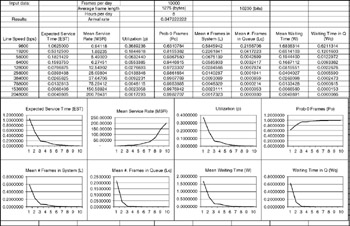
Figure 4.8: Spreadsheet Model Screen Display

4.2.4 Selecting an Operating Rate

At the beginning of this chapter, it was mentioned that queuing theory could be used to determine the operating rate of transmission lines for linking remote bridges and routers. In actuality, such usage will not produce a "magic number." Instead, the use of queuing theory can provide a range of values from which you can make a logical decision. For example, returning to Table 4.2, a line operating rate of 4800 bps is clearly unacceptable. However, what can we say concerning an operating rate of 9600 bps, 19,200 bps, 56,000 bps, etc.?

To provide some "food for thought," consider the chart marked Utilization in Figure 4.8, which shows the utilization level of the device based on the ten line operating rates that were considered . Note that at a line operating rate above the 56 Kbps to 64 Kbps range, further reductions in the utilization level of the router or bridge and an increase in the probability of zero frames in the system is essentially insignificant. Thus, you would more than likely restrict your line operating rate to a maximum of 56 to 64 Kbps in this example. To obtain a better grasp of the situation, from either Table 4.2 or Figure 4.8, note that raising the line operating rate from 64 Kbps to 128 Kbps only marginally decreases the waiting time in the queue from 0.009 seconds at 64 Kbps to 0.002 seconds at 128 Kbps. For an interactive application, the difference in the delay would not be noticeable. Thus, if you were fairly certain your application would not grow, you would probably install a digital leased line operating at 64 Kbps. Only if you anticipated further growth in transmission would you want to consider the installation of a higher speed and more costly leased line.

4.2.5 Summary

To correctly apply queuing theory to interconnecting LANs, you must first obtain knowledge about the number of transactions and the average frame size of each transaction that will flow to the other network. Once this is accomplished, you must estimate the growth in the average frame size to reflect the addition of header and trailer information required by the wide area protocol to carry your LAN frame. This then provides you with the ability to compute the average arrival rate of frames as well as the mean service rate of a remote bridge or router. Then, you can easily compute the additional queuing parameters previously discussed in this chapter and recalculate those parameters for different transmission line operating rates whose examination will enable you to select an appropriate operating rate to interconnect your LANs.

Prior to moving on to the next topic in this chapter, a few words about service time are in order. In our previous set of computations, we employed a single-channel, single-phase model based on a memory-less inter-arrival time and service time. This resulted in the model being based on the use of a negative exponential probability distribution for service time. As previously observed when we discussed the Kendall method of queuing notations, there are five basic queuing parameters that define the queuing system. Because the model we previously used was a single-channel, single-phase system and we assumed a first-in, first-out queuing method, we are basically left with considering variations in the arrival time and service time. Thus, let us focus on these two areas.

For a memory-less system, the use of a negative exponential distribution for inter-arrival time allows simple formulas to be developed to construct a queuing model. As an alternative, we could count arrivals in defined time intervals but the difference between the two over a period of time would not be significant if actual arrivals occur randomly . Because people operate computers in a random manner, this basically leaves us with the service time as a queuing system parameter to consider.

One variation in service time occurs when service time is fixed or deterministic. For Ethernet and Token Ring, a fixed service time would not be practical because frame lengths vary, resulting in a non-constant service time. However, for ATM whose cell length is fixed at 53 bytes, a deterministic service time would be more appropriate. Later in this book when we develop models to determine the performance of ATM, we will examine the use of a deterministic service time.

A second service time variation that warrants discussion occurs when the service time does not fit a negative exponential distribution but we can measure or estimate the mean service rate and its standard deviation. Then, the following set of equations would be used to model a single-channel, single-phase queuing system with Poisson arrivals and arbitrary service times:

Probability of no frames in the system:

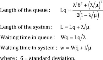
Note that if we set the standard deviation to zero, we have a model that reflects constant service times. As we will note later in this book, we can consider this model and others as a mechanism to examine ATM.