Using the Solver to Set Quantity and Pricing
When your forecasting problem contains more than one variable, you need to use the Solver add-in utility to analyze the scenario. Veterans of business school will happily remember multivariable case studies as part of their finance and operations management training. While a full explanation of multivariable problem solving and optimization is beyond the scope of this book, you don't need a business-school background to use the Solver command to help you decide how much of a product to produce, or how to price goods and services. We'll show you the basics in this section by illustrating how a small coffee shop determines which coffee beverages it should sell, and what its potential revenue will be.
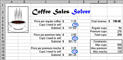
In our example, we're running a coffee shop that currently sells three beverages: regular fresh-brewed coffee, premium caffè latte, and premium caffè mocha. We currently price regular coffee at $1.25, caffè latte at $2.00, and caffè mocha at $2.25, but we're not sure what our revenue potential is and what emphasis we should give to each of the beverages. (Although the premium coffees bring in more money, their ingredients are more expensive, and they're more time-consuming to make than regular coffee.) We can make some basic calculations by hand, but we want to structure our sales data in a worksheet so that we can add to it periodically and analyze it using the Solver.
NOTE
The Solver is an add-in utility, so you should verify that it's installed on your system before you get started. If the Solver command isn't on your Tools menu, choose Add-Ins from the Tools menu, and select the Solver Add-In option in the Add-Ins dialog box. If Solver isn't in the list, you'll need to install it by running the Office Setup program again and selecting it from the list of Excel add-ins. For more information, see "Installing Add-In Commands and Wizards"
Setting Up the Problem
The first step in using the Solver command is to build a worksheet that is Solver-friendly. This involves creating a target cell to be the goal of your problem— for example, a formula that calculates total revenue that you want to maximize— and assigning one or more variable cells that the Solver can change to reach your goal. Your worksheet can also contain other values and formulas that use the target cell and the variable cells. In fact, each of your variable cells must be precedents of the target cell for the Solver to do its job. (In other words, the formula in the target cell must depend on the variable cells for part of its calculation.) If you don't set it up this way, when you run the Solver you'll get the error message, The Set Target Cell values do not converge.
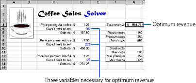
Figure 23-3 shows a simple worksheet that can be used to estimate the weekly revenue for our example coffee shop and to determine how many cups of coffee we will need to sell. Cell G4 is the target cell that calculates the total revenue that the three coffee drinks generate. The three lines that converge in cell G4 were drawn by the Trace Precedents command on the Auditing submenu of the Tools menu. They show how the formula in cell G4 depends on three other calculations for its result. (The Auditing submenu contains commands that help track the links between formulas in a worksheet.) The three variable cells in the worksheet are cells D5, D9, and D13— these are the values we want the Solver to determine when it finds an optimum solution to maximizing our weekly revenue.
ON THE WEB
The Solver.xls example is on the Running Office 2000 Reader's Corner page.
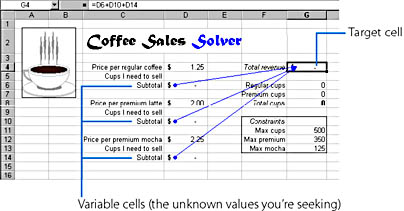
Figure 23-3. Before you use the Solver command, you need to build a worksheet that has a target cell and one or more variable cells. The Auditing submenu can help you visualize the relationship between cells.
In the bottom right corner of our screen is a list of constraints we plan to use in our forecasting. A constraint is a limiting rule or guiding principle that dictates how the business is run. For example, because of storage facilities and merchandising constraints, we're currently able to produce only 500 cups of coffee (both regular and premium) per week. In addition, our supply of chocolate restricts the production of caffè mochas to 125 per week, and a milk refrigeration limitation restricts the total production of premium coffee drinks to 350 per week.
These constraints will structure the problem, and we'll enter them in a special dialog box when we run the Solver command. Your worksheet must contain cells that calculate the values used as constraints (in this example, G6 through G8). The limiting values for the constraints are listed in cells G11 through G13. Although listing the constraints isn't necessary, it makes the worksheet easier to follow.
TIP
Name Key CellsIf your Solver problem contains several variables and constraints, you'll find it easiest to enter data if you name key cells and ranges in your worksheet by using the Define command on the Name submenu of the Insert menu. Using cell names also makes it easy to read your Solver constraints later. For more information about naming, see "Using Range Names in Functions"
Running the Solver
After you have defined your forecasting problem in the worksheet, you're ready to run the Solver add-in. The steps that follow show you how to use the Solver to determine the maximum weekly revenue for your coffee shop given the following constraints:
- No more than 500 total cups of coffee (both regular and premium)
- No more than 350 cups of premium coffee (both caffè latte and caffè mocha)
- No more than 125 caffè mochas
In addition to the maximum revenue, the Solver will tell you the optimum distribution of coffees in the three coffee groups. Complete these steps:
- Click the target cell— the one containing the formula that is based on the variable cells you want the Solver to determine— in your worksheet. In Figure 23-3, the target cell is G4.
- From the Tools menu, choose Solver.
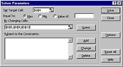
- Highlight the By Changing Cells text box. Drag the dialog box to the right so that you can see the variable cells in your worksheet. Select each of the variable cells. If the cells adjoin one another, simply select the group by dragging across the cells. If the cells are noncontiguous, hold down the Ctrl key and click each cell. This will place a comma between each cell entry in the text box.
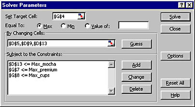
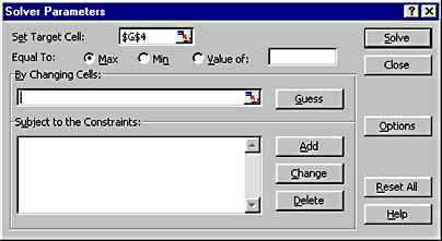
The Solver Parameters dialog box opens, as shown here. Because you clicked the target cell in step 1, the Set Target Cell text box contains the correct reference. The correct Equal To option button (Max) is also selected, because you want to find the maximum value for the cell.
In the following illustration, the three blank cells reserved for the number of coffee drinks in each category have been selected:
TIP
Use the Guess Button to Preview the ResultIf you click the Guess button, the Solver will try to guess at the variable cells in your forecasting problem. The Solver creates the guess by looking at the cells referenced in the target cell formula. Don't rely on this guess— it will often be incorrect!
NOTE
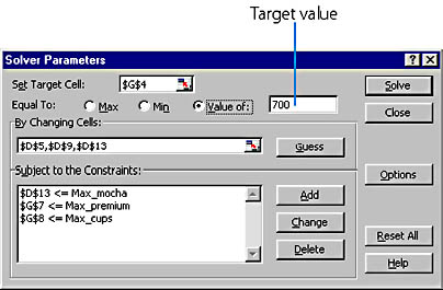
You have the option of typing a value, clicking a cell, or entering a cell name in the Constraint text box. We entered a defined cell name because it makes the constraint easier to read and modify later.