Steady-State Probabilities

[Page F-8 ( continued )]

The probabilities of .33 and .67 in our example are referred to as steady-state probabilities . The steady-state probabilities are average probabilities that the system will be in a certain state after a large number of transition periods. This does not mean the system stays in one state. The system will continue to move from state to state in future time periods; however, the average probabilities of moving from state to state for all periods will remain constant in the long run. In a Markov process, after a number of periods have passed, the probabilities will approach steady state.

Steady-state probabilities are average, constant probabilities that the system will be in a state in the future.

For our service station example, the steady-state probabilities are

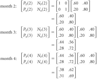
.33	=	probability of a customer's trading at Petroco after a number of months in the future, regardless of where the customer traded in month 1
.67	=	probability of a customer's trading at National after a number of months in the future, regardless of where the customer traded in month 1

Notice that in the determination of the preceding steady-state probabilities, we considered each starting state separately. First, we assumed that a customer was initially trading at Petroco, and the steady-state probabilities were computed given this starting condition. Then we determined that the steady-state probabilities were the same, regardless of the starting condition. However, it was not necessary to perform these matrix operations separately. We could have simply combined the operations into one matrix, as follows :

[Page F-9]

until eventually we arrived at the steady-state probabilities:

Direct Algebraic Determination of Steady-State Probabilities

In the previous section, we computed the state probabilities for approximately eight periods (i.e., months) before the steady-state probabilities were reached for both states. This required quite a few matrix computations . Alternatively, it is possible to solve for the steady-state probabilities directly, without going through all these matrix operations.

Notice that after eight periods in our previous analysis, the state probabilities did not change from period to period (i.e., from month to month). For example,

month 8:	[ P _p (8)	N _p (8)] = [.33	.67]
month 9:	[ P _p (9)	N _p (9)] = [.33	.67]

At some point in the future, the state probabilities remain constant from period to period.

Thus, we can also say that after a number of periods in the future (in this case, eight), the state probabilities in period i equal the state probabilities in period i + 1. For our example, this means that

[ P _p (8) N _p (8)] = [ P _p (9) N _p (9)]

In fact, it is not necessary to designate which period in the future is actually occurring. That is,

[ P _p N _p ] = [ P _p N _p ]

given steady-state conditions.

After steady state is reached, it is not necessary to designate the time period.

These probabilities are for some period, i , in the future once a steady state has already been reached. To determine the state probabilities for period i + 1, we would normally do the following computation:

However, we have already stated that once a steady state has been reached, then

[ P _p ( i + 1) N _p ( i + 1)] = [ P _p ( i ) N _p ( i )]

and it is not necessary to designate the period. Thus, our computation can be rewritten as

Performing matrix operations results in the following set of equations:

P _p = .6 P _p + .2 N _p

N _p = .4 P _p + .8 N _p

Steady-state probabilities can be computed by developing a set of equations, using matrix operations, and solving them simultaneously .

Recall that the transition probabilities for a row in the transition matrix (i.e., the state probabilities) must sum to one:

P _p + N _p = 1.0

[Page F-10]

which can also be written as

N _p = 1.0 P _p

Substituting this value into our first foregoing equation ( P _p = .6 P _p + .2 N _p ) results in the following:

P _P	=	.6 P _P + .2(1.0 P _P ) = .6 P _P + .2.2 P _P = .2 + .4 P _P
.6 P _P	=	.2
P _P	=	.2/.6 = .33

and

N _p = 1.0 P _p = 1.0 .33 = .67

These are the steady-state probabilities we computed in our previous analysis:

[ P _p N _p ] = [.33 .67]

Application of the Steady-State Probabilities

The steady-state probabilities indicate not only the probability of a customer's trading at a particular service station in the long- term future but also the percentage of customers who will trade at a service station during any given month in the long run. For example, if there are 3,000 customers in the community who purchase gasoline, then in the long run the following expected number will purchase gasoline at each station on a monthly basis:

Petroco: P _p (3,000)	=	.33(3,000)
	=	990 customers
National: N _p (3,000)	=	.67(3,000)
	=	2,010 customers

Steady-state probabilities can be multiplied by the total system participants to determine the expected number in each state in the future.

Now suppose that Petroco has decided that it is getting less than a reasonable share of the market and would like to increase its market share. To accomplish this objective, Petroco has improved its service substantially, and a survey indicates that the transition probabilities have changed to the following:

In other words, the improved service has resulted in a smaller probability (.30) that customers who traded initially at Petroco will switch to National the next month.

Now we will recompute the steady-state probabilities, based on this new transition matrix:

Using the first equation and the fact that N _p = 1.0 P _p , we have

P _P	=	.7 P _P + .2(1.0 P _P ) = .7 P _P + .2 .2 P _P
.5 P _P	=	.2
P _P	=	.2/.5 = .4

[Page F-11]

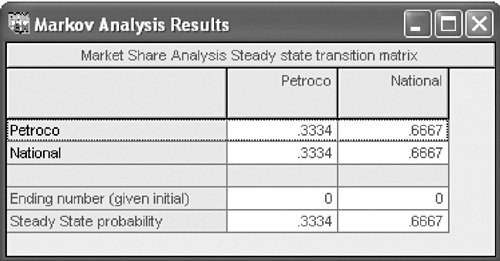
and thus

N _p = 1 P _p 1 .4 .6

This means that out of the 3,000 customers, Petroco will now get 1,200 customers (i.e., .40 x 3,000) in any given month in the long run. Thus, improvement in service will result in an increase of 210 customers per month (if the new transition probabilities remain constant for a long period of time in the future). In this situation Petroco must evaluate the trade-off between the cost of the improved service and the increase in profit from the additional 210 customers. For example, if the improved service costs $1,000 per month, then the extra 210 customers must generate an increase in profit greater than $1,000 to justify the decision to improve service.

This brief example demonstrates the usefulness of Markov analysis for decision making. Although Markov analysis does not yield a recommended decision (i.e., a solution), it does provide information that will help the decision maker to make a decision.

Markov analysis results in probabilistic information, not a decision.

Determination of Steady States with QM for Windows

QM for Windows has a Markov analysis module, which is extremely useful when the dimensions of the transition matrix exceed two states. The algebraic computations required to determine steady-state probabilities for a transition matrix with even three states are lengthy; for a matrix with more than three states, computing capabilities are a necessity. Markov analysis with QM for Windows will be demonstrated using the service station example in this section.

Exhibit F.1 shows our example input data for the Markov analysis module in QM for Windows. Note that it is not necessary to enter a number of transitions to get the steadystate probabilities. The program automatically computes the steady state. "Number of Transitions" refers to the number of transition computations you might like to see.

Exhibit F.1.

Exhibit F.2 shows the solution with the steady-state transition matrix for our service station example.

Steady-State Probabilities