NORMAL DISTRIBUTION - OTHERWISE KNOWN AS THE BELL CURVE | Six Sigma and Beyond: Statistics and Probability, Volume III

NORMAL DISTRIBUTION ” OTHERWISE KNOWN AS THE "BELL CURVE"

Figure 16.12 shows a typical normal curve with a mean and a standard deviation.

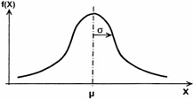
Figure 16.12: A typical normal curve.

TYPICAL COMMENTS ABOUT THE NORMAL CURVE

Most important distribution function in statistics.
Many populations are normally distributed.
Some distributions are made normal by changing variables .
Normal can approximate discrete binomial distribution.
Central Limit Theory ’ distribution of means is normal.
Confidence limits are based on normal parameters.

Only two statistical parameters describe distribution:

¼	=	Mean
ƒ	=	Standard Deviation

Normal Probability Density Function is symmetric about mean.

Note	Mode = Mean = Median.

It turns out that the probability density function for variable x may be shown as in Figure 16.13.

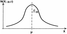
Figure 16.13: Probability density function for random variable x.

Mathematically this is written as:

with the following population parameters: ¼ = population mean, ƒ ² = variance of population, ƒ = standard deviation of population, RV - ˆ < x < ˆ , inflection points at x = ¼ ± ƒ .

It is very important to realize that the area under the pdf is always unity even though the mean and standard deviation may differ . This is shown in Figures 16.13 and 16.14, respectively. Also in Figure 16.14 the probability density function is shown with different means and fixed standard deviation whereas the Figure 16.15 shows the probability density function with different means and/or standard deviations.

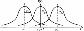
Figure 16.14: Probability density function with different means and same standard deviation.

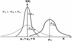
Figure 16.15: Probability density with different means and/or standard deviation.

In addition, the normal curve may be represented as a cumulative distribution function. Its mathematical notation is

This is shown pictorially in Figure 16.16.

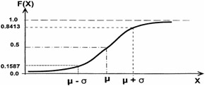
Figure 16.16: Cumulative distribution function.

A word of caution ” Any area of specified region under probability density function may be identified and calculated. However, the calculation cannot be a direct integration. Rather, because the normal probability function cannot be integrated directly, standardized cumulative distributions are tabulated. When those tabulations are figured out, the reader must be very careful because not all tables give the same "area" of p.d.f. For example, some tables give S-CD values in interval: p (0 Z Z ) and some tables give S-CD values of upper tail: P (Z _o Z ˆ ).

DIFFERENTIAL EQUATION (DE)

The normal distribution functions can be generated from the first order homogeneous differential equation having a non-constant coefficient:

where X is the independent random variable, Y is the dependent random variable (p.d.f.), is the mean, and s ² is the variance (units of X ² ).

Separation of variables yields:

Solution of DE: In Y = -(X - ) ² /(2s ² )

Given the constraint that the area of the integral is unity, Y{X)dX 1. (The units of the probability density Y are the inverse of X.) It can be shown that the amplitude is adjusted so

STANDARDIZED RANDOM VARIABLES ” TABULATED FUNCTION

Any random variable X can be transformed into a normalized (non-dimensional) standardized random variable Z

Subtracting the mean shifts mean of RV to origin: Z = 0.
Dividing by standard deviation makes variance unity and eliminates physical units.

This transformation is the function typically tabulated and plotted in statistics textbooks .

STANDARDIZED NORMAL DISTRIBUTION (SND)

Probability density function for the random variable Z:

where mean: ¼ _z = 0, standard deviation: ƒ _z = 1, and RV - ˆ z ˆ . Pictorially this can be shown as in Figure 16.17. At the mean value, z = 0, the pdf is N (0; 0, 1) = 0.4. Also, this figure shows the unstandardized distribution as a comparison.

Figure 16.17: Standardized and unstandardized normal function” (a) unstandardized distribution, (b) standardized distribution.

On the other hand, the cumulative distribution function (area under standardized probability density function for a given interval) of the standardized normal distribution may be presented mathematically as:

The graph is shown in Figure 16.18. Recall, however, that the probability for all continuous random variables can only be determined in terms of an interval such as P(Z ₁ Z Z ₂ ).

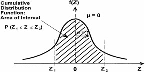
Figure 16.18: Cumulative distribution function ” area of interval.

Tabulated possibilities include:

P(- ˆ Z Z )
P(0 Z Z )
P(Z Z ˆ )

Figure 16.19 shows the tabulated distribution function for leading tail.

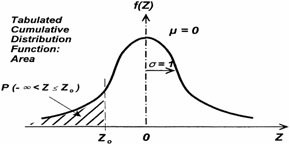
Figure 16.19: Tabulated cumulative distribution function ” leading tail.

Tabulated Values (Leading Tail): P (- ˆ z z )
Z = -3	p (- ˆ Z -3) = 0.00135
Z = -2	p (- ˆ Z -2) = 0.0228
Z = -1	p (- ˆ Z -1) = 0.1587
Z = 0	p (- ˆ Z 0) = 0.5000
Z = 1	p (- ˆ Z 1) = 0.8413
Z = 2	p (- ˆ Z 2) = 0.9772
Z = 3	p (- ˆ Z 3) = 0.99865

Figure 16.20 shows the tabulated cumulative distribution function under a specific interval area.

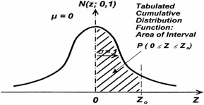
Figure 16.20: Tabulated cumulative distribution function ” area of specific interval.

Tabulated Values (Center .Interval): P(0 Z Z )
Z = 0.0:	P(0 Z 0.0) = 0.0000
Z = 0.5:	P(0 Z 0.5) = 0.1915
Z = 1.0:	P(0 Z 1.0) = 0.3413
Z = 1.5:	P(0 Z 1.5) = 0.4332
Z = 2.0:	P(0 Z 2.0) = 0.4772
Z = 2.5:	P(0 Z 2.5) = 0.4938
Z = 3.0:	P(0 Z 3.0) = 0.4987

Finally, the cumulative distribution function with a trailing tail is shown in Figure 16.21.

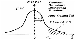
Figure 16.21: Standardized normal distribution with trailing tail.

Tabulated Values (Trailing Tail): P(Z Z ˆ )
Z = 0.0:	P(0.0 Z ˆ ) = 0.5000
Z = 0.5:	P(0.5 Z ˆ ) = 0.3085
Z = 1.0:	P(1.0 Z ˆ ) = 0.1587
Z = 1.5:	P(1.5 Z ˆ ) = 0.0668
Z = 2.0:	P(2.0 Z ˆ ) = 0.0228
Z = 2.5:	P(2.5 Z ˆ ) = 0.00621
Z = 3.0:	P(3.0 Z ˆ ) = 0.00135
Z = 4.0:	P(4.0 Z ˆ ) = 0.0000317

Example 1

Given: The life of a particular electronic component is normally distributed with a mean ¼ = 200 hours and a standard deviation of a ƒ _x = 20 hours.

Find: The expected percentage of components requiring replacement at or before 150 hours.

Standard random variable:

That is to say, the specified replacement time (150 hr) is 2.5 ƒ below the mean. Cumulative probability distribution:

P(- ˆ X 150) = p (- ˆ Z -2.5) = 0.00621

Hence, only 0.621% of components are expected to be replaced at or before 150 hours. Because SND is symmetric, you can use either of these tabulations:

P(- ˆ < Z -2.5) = 0.00621 = P(2.5 Z ˆ ) = 0.00621

This may be represented in a pictorial form as in Figure 16.22.

Figure 16.22: Electronic components in a symmetrical format of the distribution.

Example 2

Given: A particular engine component is being manufactured having a tension X that is found to be normal distribution with a mean ¼ = 60 N and a standard deviation of ƒ _x = 10 N. The manufacturing specifications for the tension of this component are 45 to 70 N.

Find: The percentage of manufactured parts expected to be within specification. Standard random variable limits:

That is to say, the specifications are within 1.5 ƒ and + 1.0 ƒ of the manufactured mean. This can be shown in Figure 16.23.

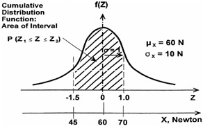
Figure 16.23: Area of interval ” cumulative distribution function.

Determine net probability:

P(45 X 70) = P(-1.5 Z 1.0)

Cumulate areas consistent with tabulation given. Assume given trailing tail tabulation:

P(-1.5 Z 1.0)	= P(-1.5 Z ˆ ) - P(1.0 Z ˆ )
	= [1 - P(1.5 Z ˆ )] - P(1.0 Z ˆ )
	= [1 - 0.0668] - 0.1587 = 0.7745

Hence, 77.45% of the currently manufactured components are expected to "meet spec." This is shown in Figure 16.24.

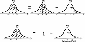
Figure 16.24: The graphical progression in figuring out the components of "meeting specifications."

So, the reader by now has figured out that at any point in the curve we can indeed find the area provided we know the mean and the standard deviation.

Figure 16.25 shows the area under the curve in percentage for the traditional mean equals zero and standard deviation of one for the three deviations about the mean.

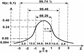
Figure 16.25: Percent area under the SND curve.