A1.6 Tests of Hypotheses

A1.6 Tests of Hypotheses

A1.6.1 Basic Principles

Many of the basic decisions confronting software engineering are binary; there are just two distinct courses of actions that can be taken. If the software engineer had complete information, then the appropriate course of action would be obvious. The purpose of statistics is to provide some information that can be used in making a reasonable decision between the two possible actions. The possible perceived states of Nature are said to be hypotheses about Nature. Further, each of the states is said to be a simple hypothesis. It is possible to form a set of simple hypotheses into a composite hypothesis that will be true if some of the simple hypotheses are true.

One of the major challenges in the field of research is the formulation of questions that have answers. We might, for example, formulate a hypothesis that the population on which a random variable X is defined has a mean of 50. We could then design an experiment that would test this simple hypothesis. In this process we would collect a sample set of observations, compute the mean of the sample, compare this sample mean with the population mean, and either accept the simple hypothesis or reject it. If, on the other hand, we were to form the hypothesis that X is normally distributed, then we would have a composite hypothesis. This is so because a normal distribution is defined by its mean and variance. The actual composite hypothesis is that X ~ N(μ,σ). To specify a normal distribution, we must know both the mean and the variance.

In general then, the strategy is to partition the decision space into two actions A and B, depending on two alternate hypotheses H₀ and H₁. The first hypothesis, H₀, is often called the null hypothesis, in that it very often means that we will not change our current strategy based on the acceptance of this hypothesis. Most experimental designs are centered only on H₀. That is, we will accept H₀ or we will reject H₀, which implies the tacit acceptance of H₁. We might wish, for example, to test the value of a new design methodology such as object-oriented (O-O) programming. We would formulate a hypothesis H₀ that there would be no significant difference between an ad hoc program design and O-O with respect to the number of embedded faults in the code as observed in the test process. We would then conduct the experiment and if we found that there were no differences in the two design methodologies, we would then accept the null hypothesis H₀. If, on the other hand, we found significant differences between the two groups, we would then reject the null hypothesis in favor of H₁.

In arriving at a decision about the null hypothesis H₀, two distinct types of error can arise. We can be led to the conclusion that H₀ is false when, in fact, it is true. This is called a Type I error. Alternatively, we can accept H₀ as true when the alternate hypothesis H_l is true. This is called a Type II error. There will always be some noise in the decision-making process. This noise will obscure the true state of Nature and lead us to the wrong conclusion. There will always be a nonzero probability of our making a Type I or Type II error. By convention, α will be the probability of making a Type I error and β the probability of making a Type II error. From the standpoint of responsible science, we would much rather make a Type II error than a Type I error. Far better is it to fail to see a tenuous result than it would be to be led to the wrong conclusion from our experimental investigation.

At the beginning of each experiment, the values of α and β are determined by the experimenter. These values remain fixed for the experiment. They do not change based on our observations. Thus, we might choose to set α < 5.05. That means that we are willing to accept a 1-in-20 chance that we will make a Type II error. A test of significance is a statistical procedure that will provide the necessary information for us to make a decision. Such a statistical test can, for example, show us that our result is significant at α < 0.035. If we have established our a priori experimental criterion at α < 0.05, then we will reject the null hypothesis. As a matter of form, a test is either significant at our a priori level of a or it is not. If we were to observe two tests, one significant at α < 0.03 and the other at α < 0.02, we would never report the former test as more significant than the latter. They are both significant at the a priori level of α < 5.05.

The determination of the probability β of making a Type I error is a little more tenuous. It is dependent on the statistical procedures that we will follow in an experiment. We might, for example, be confronted in an experimental situation with two alternative procedures or tests. If two tests of simple H₀ against simple H_l have the same α, the one with the smaller β will dominate and is the preferred test of the two. It is the more powerful of the two tests. In general then, the power of a test is the quantity 1-β.

It is possible to conceive of two simple experiments A and B that are identical in every respect except for the number of observations in each. B might have twice as many observations in its sample as A. Within a given test of significance, the test for B will be more powerful than that for A. It would seem, then, that the best strategy is to design large experiments with lots of observations. This is not desirable in software engineering for two totally different reasons. First, we will learn that experimental observations in software engineering are very expensive. More observations are not economically better. Even worse is the prospect that we run the risk of proving the trivial. As a test increases in power, the more resolving power it will have on any differences between two groups, whether these differences are related to the experiment or not. More is not better. Rather, we must identify a procedure that will allow us to determine just how many observations we will need for any experiment. Intuitively, in any experiment there is the signal component that represents the information that we wish to observe. There is also a noise component that represents information added to the experiment by Nature that will obscure our signal event. The ratio of the signal strength to the noise component will be a very great determinant in our evolving sense of experimental design.

A1.6.2 Test on Means

The tests of hypotheses in statistics are rather stereotyped. Experiments, in general, are formulated around hypotheses that relate either to measures of central tendency (mean) or to measures of variation. The formulation of hypotheses in this manner is a large part of the craft of experimental design. Any unskilled person can ask questions. Most questions, however, do not have scientific answers. It takes a well-trained person in experimental design to postulate questions that have answers.

Hypothesis testing in its most simple form occurs when we have identified an experimental group that we think is different from (or similar to) a control group, either because of some action that we have taken or because of some ex post facto evidence that we have collected. If the members of the experimental group sample are different from the population, then the statistics describing our experimental group will differ from the control group. In particular, the mean of the experimental group, , will be different from the mean of the control group, . We will conveniently assume that the samples are drawn from normally distributed populations with means of μ₁ and μ₂ and a common variance of σ². The null hypothesis for this circumstance is:

H₀: μ₁ - μ₂ = 0

The case for the alternate hypothesis is not so clear. Depending on the nature of the experimental treatment, there are three distinct possibilities for H₁ as follows:

If we now consider the new random variables , where and are sample means of the two populations, this sum also has a normal distribution, its mean is μ₂ - μ₁, and its standard deviation is:

Then:

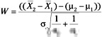
is distributed normally such that W ~ N(0,1).

Now, if and are random variables representing the sample variances, then and have the χ² distribution with n₁+1 and n₂ + 1 degrees of freedom. Their sum

also has the χ² distribution with n₁ +n² - 2 degrees of freedom. Therefore:

has the t distribution with n₁ + n₂ - 2 degrees of freedom. Substituting for W and V we have:

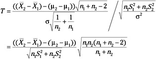
We will assume now that the null hypothesis is true. This being the case, μ₁ - μ₂ = 0. The actual value of the t distribution that will be used as a criterion value of the acceptance of the null hypothesis will be derived from:

Now let us return to the three alternate hypotheses to understand just how to construct a criterion value for the test of the null hypothesis from the t distribution. First, let us set an a priori experimental value for a < 0.05. If we wish to employ , then we wish to find a value a such that Pr(T > a) = 0.05 or

for the t distribution with n₁ + n₂ - 2 degrees of freedom. To simplify this notation for future discussions, let us represent this value as t(n₁ + n₂ - 2, 1- α). In the case that we wish to use the alternate hypothesis , we would use precisely the same value of t. Tests of this nature are called one-tailed t tests in that we have set an upper bound a on the symmetrical t distribution.

In the special case for the second hypothesis , we have no information on whether μ₁ > μ₂ or μ₁ < μ₂; consequently, we are looking for a value of a such that Pr(-a < T > a) = 0.05. Given that the t distribution is symmetrical, Pr(-a < T > a) = 0.05 is equal to 2Pr(T₁ > a). Thus, for this two-tailed t test we will enter the table for .