A1.7 Introduction to Modeling
|
|
A1.7 Introduction to Modeling
An important aspect of statistics in the field of software engineering will be for the development of predictive models. In this context we will have two distinct types of variables. We will divide the world into two sets of variables: independent and dependent. The objective of the modeling process is to develop a predictive relationship between the set of independent variables and the dependent variables. Independent variables are called such because they can be set to predetermined values by us or their values may be observed but not controlled. The dependent or criterion measures will vary in accordance with the simultaneous variation in the independent variables.
A1.7.1 Linear Regression
There are a number of ways of measuring the relationships among sets of variables. Bivariate correlation is one of a number of such techniques. It permits us to analyze the linear relationship among a set of variables, two at a time. Correlation, however, is just a measure of the linear relationship, and nothing more. It will not permit us to predict the value of one variable from that of another. To that end, we will now explore the possibilities of the method of least squares or regression analysis to develop this predictive relationship.
The general form of the linear, first-order regression model is:
y = β0+β1x + ε
In this model description, the values of x are the measures of this independent variable. The variable y is functionally dependent on x. This model will be a straight line with a slope of β1 and an intercept of β0. With each of the observations of y there will be an error component ε that is the amount by which y will vary from the regression line. The distributions of x and y are not known, nor are they relevant to regression analysis. We will, however, assume that the errors ε do have a normal distribution.
In a more practical sense, the values of ε are unknown and unknowable. Hence, the values of y are also unknown. The very best we can do is to develop a model as follows:
ŷ = b0+b1x
where b0 and b1 are estimates of β0 and β1, respectively. The variable ŷ represents the predicted value of y for a given x.
Now let us assume that we have at our disposal a set of n simultaneous observations (x1,y1),(x2,y2),...,(xn,yn) for the variables x and y. These are simultaneous in that they are obtained from the same instance of the entity being measured. If the entity is a human being, then (xi,yi) will be measures obtained from the ith person at once. There will be many possible regression lines that can be placed through this data. For each of these lines, εi in
yi = β0 + β1xi + εi
will be different. For some lines, the sum of the εis will be large and for others it will be small. The particular method of estimation that is used in regression analysis is the method of least squares. In this case, the deviations εi of yi will be:
![]()
The objective now is to find values of b0 and b1 that will minimize S. To do this we can differentiate first with respect to β0 and then β1 as follows:
![]()
![]()
The next step is to set each of the differential equations equal to zero, and substitute the estimates b0 and b1 for β0 and β1:
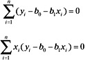
Performing a little algebraic manipulation, we obtain:
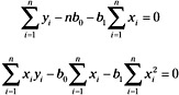
These, in turn, yield the set of equations known as the normal equations:
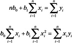
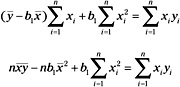
These normal equations will first be solved for b0 as follows:
![]()
Next, we will solve for b1 as follows:
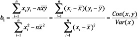
A1.7.1.1 The Regression Analysis of Variance.
It is possible to use the least squares fit to fit a regression line through data that is perfectly random. That is, we may have chosen a dependent variable and an independent variable that are not related in any way. We are now interested in the fact that the independent variable varies directly with the independent variable. Further, a statistically significant amount of the variation in the independent variable should be explained by a corresponding variation in the independent variable. To study this relationship we will now turn our attention to the analysis of variance (ANOVA) for the regression model.
First, observe that the residual value, or the difference between the predicted value ŷi and the observed value yi can be partitioned into two components as follows:
![]()
Now, if the two sides are squared and summed across all observed values, we can partition the sum of squares about the regression line (yi-ŷi)2 as follows:
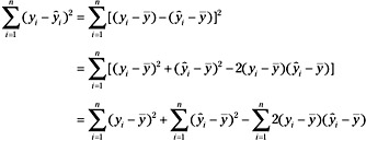
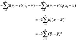
Now observe that:
![]()
Thus, the last term in the equations above can be written as:
If we substitute this result into the previous equation, we obtain:
![]()
which can be rewritten as:
![]()
From this equation we observe that the total sum of squares about the mean (SStot) can be decomposed into the sum of squares about the regression line (SSres) and the sum of squares due to regression (SSreg):
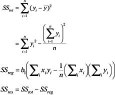
In essence, the above formula shows how the total variance about the mean of the dependent variable can be partitioned into the variation about the regression line, residual variation, and the variation directly attributable to the regression. We will now turn our attention to the analysis of this variation or the regression ANOVA. The basic question that we ask in the analysis of variance is whether we are able to explain a significant amount of variation in the dependent variable or is the line we fitted likely to have occurred by chance alone.
We will now construct the mean squares of the sums of squares due to regression and due to the residual. This will be accomplished by dividing each term by the degrees of freedom of each term. This term is derived from the number of independent sources of information needed to compile the sum of squares. The sum of squares total has (n - 1) in that the sum of ![]() must sum to zero. Any of the combinations of (n - 1) terms are free to vary but the nth term must always have a value such that the sum is zero. The sum of squares due to regression can be obtained directly from a single function b1 of the yis. Thus, this sum of squares has only one degree of freedom. The degrees of freedom, then, for the residual sum of squares can be obtained by subtraction and is (n - 2). Thus, MSreg = SSreg / 1 and MSres = SSres / (n - 2). Now let us observe that SSreg and SSres both have the χ2 distribution. Therefore:
must sum to zero. Any of the combinations of (n - 1) terms are free to vary but the nth term must always have a value such that the sum is zero. The sum of squares due to regression can be obtained directly from a single function b1 of the yis. Thus, this sum of squares has only one degree of freedom. The degrees of freedom, then, for the residual sum of squares can be obtained by subtraction and is (n - 2). Thus, MSreg = SSreg / 1 and MSres = SSres / (n - 2). Now let us observe that SSreg and SSres both have the χ2 distribution. Therefore:
![]()
has the F distribution with 1 and (n - 2) degrees of freedom, respectively. Therefore, we can determine whether there is significant variation due to regression, if the F ratio exceeds our a priori experiment wise significance criterion of α > 0.05 from the definition of the f distribution:
![]()
where g(x)s is defined in Section A1.4.4. As with the t distribution, actually performing this integration for each test of significance that we wished to perform would defeat the most determined researchers among us. The critical values for F(df1,df2, 1-α) can be obtained from the tables in most statistics books.
The coefficient of determination R2 is the ratio of the total sum of squares to the sum of squares due to regression, or:
![]()
It represents the proportion of variation about the mean of y explained by the regression. Frequently, R2 is expressed as a percentage and is thus multiplied by 100.
A1.7.1.2 Standard Error of the Estimates.
As noted when we computed the mean of a sample, this statistic is but an estimate of the population mean. Just how good an estimate it is, is directly related to its standard error. Therefore, we will now turn our attention to the determination of the standard error of the slope, the intercept, and the predicted value for y.
The variance of b1 can be established as follows:
![]()
The standard error of b1 is simply the square root of the variance of b1 and is given by:
![]()
In most cases, however, we do not know the population variance. In these cases we will compute the estimated standard error of b1 as follows:
![]()
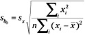
The variance of b0 can be obtained from:
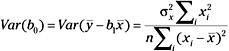
Following the discussion above for b1, the standard error of b0 is then given by:
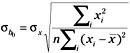
By substituting the sample standard deviation for the population parameter, we can obtain the estimated standard error for b0 as follows:
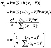
To obtain the standard error of ŷ, observe that:
![]()
The variance of ŷ can then be obtained from:
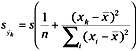
As before, substituting the sample variance for the population parameter, the estimated standard error of ŷ is then given by:
A1.7.1.3 Confidence Intervals for the Estimates.
Once the standard error of the estimate for b0 has been established, we can compute the (1-α) confidence interval for b0 as follows:
![]()
We may wish to test the hypothesis that β0 = 0 against the alternate hypothesis that β0 ≠ C, in which case we will compute the value
![]()
to see whether it falls within the bounds established by ![]() . In a similar fashion, the (1-α) confidence interval for b1 is as follows:
. In a similar fashion, the (1-α) confidence interval for b1 is as follows:
![]()
Sometimes it will occur that we are interested in whether the slope b1 has a particular value, say 0 perhaps. Let γ be the value that we are interested in. Then, the null hypothesis is H0: β0 = γ and the alternate hypothesis is H1: β0 ≠ γ. We will compute the value
![]()
to see whether |t| falls within the bounds established by ![]() .
.
We would now like to be able to place confidence intervals about our estimates for each of the predicted values of the criterion variable. That is, for each observation xj, the model will yield a predicted ŷk. We have built the regression model for just this purpose. We intend to use it for predicting future events. If the model is good, then our prediction will be valuable. If only a small portion of the variance of y about its mean is explained by the model, the predictive value of the model will be poor. Thus, when we use the model for predictive purposes, we will always compute the experimentally determined (1-α) confidence limits for the estimate:
![]()
The purpose of this section has been to lay the statistical foundation that we will need for further discussions on modeling.
|
|
EAN: 2147483647
Pages: 139