Data Mining Examples

For many of us, the best way to learn something is by doing it. This is especially true for technical folks, and even more so for data mining. You really need to work through the SQL 2005 Data Mining Tutorial before you run through this example. This will give you a chance to get familiar with the tools and the user interface, which will make these examples easier to understand and follow. If you havent already done so, please take the time to go work through the data mining tutorials now.

In this section we start out with a simple example to get a feel for the data mining tool environment and the data mining process. In fact, the first example is so simple that its case set of economic data can be presented on a single page. Then we dig into a more detailed example based on the Adventure Works Cycles data mining tutorial data. Both of these examples will follow the general flow of the data mining process presented in the previous section.

Case Study: Classifying Cities

This first example is a small, simplified problem designed to provide a clear understanding of the process. The dataset has only 48 cases totalnot nearly enough to build a robust data mining model. However, the small size allows us to examine the inputs and outputs to see if the resulting model makes sense. The scenario is based on a large non-governmental organization with a mission and operations much like that of the World Bank:

(T)o fight poverty and improve the living standards of people in the developing world. It is a development Bank that provides loans, policy advice, technical assistance and knowledge sharing services to low and middle income countries to reduce poverty. The Bank promotes growth to create jobs and to empower poor people to take advantage of these opportunities. ( http://web.worldbank.org/ )

Classifying Cities: Business Opportunity

The data miner on the Banks DW/BI team held meetings with key directors and managers from around the organization to identify business opportunities that are supported by available data and can be translated into data mining opportunities. During these meetings it became clear that there were not enough resources to properly customize the Banks programs. The Bank had historically focused its efforts to provide financial aid at the country level. Several economists felt that targeting policies and programs at the city level would be more effective, allowing for the accommodation of unique regional and local considerations that are not possible at the country level.

A switch to the city level would mean the people who implemented the Banks programs would need to deal with potentially thousands of cities rather than the 208 countries they were working with around the world. This switch would significantly expand the complexities of managing the economic programs in an organization that was already resource limited.

The group discussed the possibility of designing programs for groups of cities that have similar characteristics. If there were a relatively small number of city groups, the economic analysts felt it would be possible to design the appropriate programs.

Classifying Cities: Data Understanding

During the meetings, there was discussion about what variables might be useful inputs. The analysts had a gut feel for what the city-groups might be, and some initial guesses about which variables would be most important and how they could be combined. The group came up with a list of likely variables. The data miner combed through the organizations databases to see if these inputs could be found, and to see what other relevant information was available. This effort turned up 54 variables that the organization tracked, from total population to the number of fixed line and mobile phones per 1,000 people. This wealth of data seemed too good to be true, and it was. Further investigation revealed that much of this data was not tracked at the city level. In fact, there were only ten city-level variables available. The data miner reviewed this list with the business folks and the group determined that of the ten variables, only three were reliably measured. Fortunately, the group also felt these three variables were important measures of a citys economic situation. The three variables were average hourly wages (local currency), average hours worked per year, and the average price index.

At this point, the data miner wrote up a description of the data mining opportunity, its expected business impact, and an estimate of the time and effort it would take to complete. The project was described in two phases; the goal of the first phase was to develop a model that clusters cities based on the data available. If this model made sense to the business folks, phase two would use that model to assign new cities to the appropriate clusters as they contact the bank for financial support. The data mining opportunity description was reviewed by the economists and all agreed to proceed.

Classifying Cities: Data Preparation

The data miner reviewed the dataset and realized it needed some work. First, the average hourly wages were in local currencies. After some research on exchange rates and discussion with the economists to decide on the appropriate rates and timing, the data miner created a package to load and transform the data. The package extracted the data from the source system and looked up the exchange rate for each city and applied it to the wages data. Because the consumer price data was already indexed relative to Zurich, using Zurich as 100, this package also indexed the wage data in the same fashion. Finally, the package wrote the updated dataset out to a separate table. The resulting dataset to be used for training the cluster model, containing three economic measures for 46 cities around the world, is shown in Table 10.3.

Table 10.3: The City Economic Data Training Set After Data Preparation

OBS.	CITY NAME	AVG WORK HRS	PRICE INDEX	WAGE INDEX
1	Amsterdam	1714	65.6	49
2	Athens	1792	53.8	30.4
3	Bogota	2152	37.9	11.5
4	Bombay	2052	30.3	5.3
5	Brussels	1708	73.8	50.5
6	Buenos Aires	1971	56.1	12.5
7	Cairo	NULL	37.1	NULL
8	Caracas	2041	61	10.9
9	Chicago	1924	73.9	61.9
10	Copenhagen	1717	91.3	62.9
11	Dublin	1759	76	41.4
12	Dusseldorf	1693	78.5	60.2
13	Frankfurt	1650	74.5	60.4
14	Geneva	1880	95.9	90.3
15	Helsinki	1667	113.6	66.6
16	Hong Kong	2375	63.8	27.8
17	Houston	1978	71.9	46.3
18	Jakarta	NULL	43.6	NULL
19	Johannesburg	1945	51.1	24
20	Kuala Lumpur	2167	43.5	9.9
21	Lagos	1786	45.2	2.7
22	Lisbon	1742	56.2	18.8
23	London	1737	84.2	46.2
24	Los Angeles	2068	79.8	65.2
25	Luxembourg	1768	71.1	71.1
26	Madrid	1710	93.8	50
27	Mexico City	1944	49.8	5.7
28	Montreal	1827	72.7	56.3
29	Nairobi	1958	45	5.8
30	New York	1942	83.3	65.8
31	Nicosia	1825	47.9	28.3
32	Oslo	1583	115.5	63.7
33	Panama	2078	49.2	13.8
34	Paris	1744	81.6	45.9
35	Rio de Janeiro	1749	46.3	10.5
36	Sao Paulo	1856	48.9	11.1
37	Seoul	1842	58.3	32.7
38	Singapore	2042	64.4	16.1
39	Stockholm	1805	111.3	39.2
40	Sydney	1668	70.8	52.1
41	Taipei	2145	84.3	34.5
42	Tel Aviv	2015	67.3	27
43	Tokyo	1880	115	68
44	Toronto	1888	70.2	58.2
45	Vienna	1780	78	51.3
46	Zurich	1868	100	100

Note 

This data actually comes from the Economics Research Department of the Union Bank of Switzerland. The original set contains economic data from 48 cities around the globe in 1991. It has been used as example data for statistics classes and can be found on many web sites. Try searching for cities prices and earnings economic (1991) globe.

Observe that two of the cities are missing data. The data miner might opt to exclude these cities from the dataset, or include them to see if the model can identify them as outliers. This would help spot any bad data that might come through in the future.

Classifying Cities: Model Development

Because the goal in the first phase was to identify groups of cities that have similar characteristics, and those groupings were not predetermined, the data miner decided to use the Microsoft Clustering algorithm. After creating a new Analysis Services project in BI Studio and adding a data source and data source view that included the City dataset, the data miner right-clicked on the Mining Structures folder and selected New Mining Structure. This opened the Data Mining Wizard to create a new mining structure. The wizard asks if the source is relational or OLAP, and then it asks which data mining technique should be used. The data miner chose Microsoft Clustering and specified the city name as the key and the other columns as input, checking the Allow drill through box on the final wizard screen. After the wizard was finished, the data miner clicked the Mining Model Viewer tab, which forced the build/ deploy/process steps. When this whole process completed, BI Studio presented the cluster diagram shown in Figure 10.7.

At first glance, this diagram isnt that helpful. Without knowing anything about the problem, the Microsoft Clustering algorithm is limited to names like Cluster 1 and Cluster 2. At this point, the data miner can explore the model by using the other tabs in the Mining Model Viewer tab, and by using the drillthrough feature to see which cities have been assigned to which nodes. The data miner can also use the Microsoft Mining Content Viewer to examine the underlying rules and distributions. The data in Table 10.4 is grouped by cluster and was created by drilling through each cluster and copying the underlying list into a spreadsheet.

Table 10.4: City Economic Data Listed by Cluster

CLUSTER	CITY NAME	AVG WORK HRS	PRICE INDEX	WAGE INDEX
Cluster 1	Bogota	2152	11.5	37.9
	Bombay	2052	5.3	30.3
	Buenos Aires	1971	12.5	56.1
	Caracas	2041	10.9	61.0
	Kuala Lumpur	2167	9.9	43.5
	Lagos	1786	2.7	45.2
	Mexico City	1944	5.7	49.8
	Nairobi	1958	5.8	45.0
	Panama	2078	13.8	49.2
	Rio de Janeiro	1749	10.5	46.3
	Sao Paulo	1856	11.1	48.9
Cluster 2	Athens	1792	30.4	53.8
	Hong Kong	2375	27.8	63.8
	Johannesburg	1945	24.0	51.1
	Lisbon	1742	18.8	56.2
	Nicosia	1825	28.3	47.9
	Singapore	2042	16.1	64.4
Cluster 7	Seoul	1842	32.7	58.3
	Tel Aviv	2015	27.0	67.3
Cluster 6	Houston	1978	46.3	71.9
	Los Angeles	2068	65.2	79.8
	Taipei	2145	34.5	84.3
Cluster 4	Brussels	1708	50.5	73.8
	Chicago	1924	61.9	73.9
	Dusseldorf	1693	60.2	78.5
	Frankfurt	1650	60.4	74.5
	Luxembourg	1768	71.1	71.1
	Montreal	1827	56.3	72.7
	New York	1942	65.8	83.3
	Sydney	1668	52.1	70.8
	Toronto	1888	58.2	70.2
	Vienna	1780	51.3	78.0
Cluster 5	Amsterdam	1714	49.0	65.6
	Copenhagen	1717	62.9	91.3
	Dublin	1759	41.4	76.0
	London	1737	46.2	84.2
	Madrid	1710	50.0	93.8
	Paris	1744	45.9	81.6
Cluster 3	Geneva	1880	90.3	95.9
	Helsinki	1667	66.6	113.6
	Oslo	1583	63.7	115.5
	Stockholm	1805	39.2	111.3
	Tokyo	1880	68.0	115.0
	Zurich	1868	100.0	100.0
Cluster 8	Cairo			37.1
	Jakarta			43.6

Table 10.4 has a few interesting items. The clusters seem to make general sense given a basic understanding of the world economic situation in 1991. Many of the poorer cities of South and Central America and Africa ended up in Cluster 1. The two cities that had only price data, Cairo and Jakarta, are on their own in Cluster 8, and that cluster was drawn a distance from the other six in Figure 10.7. Cluster 8 seems to be the data anomalies cluster. Beyond this, its difficult to see what defines a given cluster from the data table. The underlying rules are too complex to reverse engineer by sight. The Microsoft Mining Content Viewer can help by revealing the equations that determined each cluster, but a graphical representation will usually reveal much more than written equations.

Figure 10.8 converts the data from Table 10.4 into a graphical form. Each city is grouped by cluster along the X axis, with work hours plotted on the left Y axis and wage and price indexes on the right Y axis. The order of the clusters was determined by starting with Cluster 1 in Figure 10.7 and following the links. This graph allows the viewer to get a better sense for what makes up the clusters.

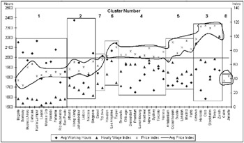
Figure 10.8: A graphical view of the city clusters

Even though Figure 10.8 is a bit busy, it helps clarify the commonalities within each cluster. The cloud-like circles in Figure 10.8 highlight the Price Index data points. The horizontal line in the graph indicates the average Price Index of about 69.2. Clusters 6, 4, and 3 on the upper part of the right side of the graph have a Price Index above average, while Clusters 1, 2, and 7 on the left side are all below average. This graph also makes it easier to identify the characteristics of the individual clusters. For example, Cluster 4 includes cities whose wages are relatively high, with prices that are at the low end of the high price range, and relatively low work hours. These are the cities that make up the day-to-day workforce of their respective countrieswe might call this cluster the Heartland cities. Cluster 1, on the other hand, has extremely low wages, higher work hours than most, and relatively lower prices. These are the newly developing cities where labor is cheap and people must work long hours to survive. You might call this cluster the Hard Knock Life cities. The Bank would likely call it something a bit more politically correct, like the Developing Cities cluster. As we mentioned earlier, good names can help crystallize the defining characteristics of each cluster.

Classifying Cities: Model Validation

Some data mining models are easier to test than others. For example, when youre building a prediction model, you can create it based on one historical dataset and test it on another. Having historical data means you already know the right answer, so you can feed the data through the model, see what value it predicts, and compare it to what actually happened .

In the City cluster example, validating the model is not so straightforward. You dont know the classification ahead of time, so you cant compare the assigned cluster with the right clusterthere is no such thing as right in this case. Validation of this model came in two stages. First, the data miner went back to the economic analysts and reviewed the model and the results with them. This was a reasonableness test where the domain experts compared the model with their own understanding of the problem. The second test came when the model was applied to the original business problem. In this case the team monitored the classification of new cities to make sure they continued to stand up to the reasonableness test. Ultimately, the question was Do the classifications seem right, and do they help simplify how the organization works at the city level? Is it easier and more effective to work with eight clusters rather than 46 (or 4,600) cities?

Classifying Cities: Implementation

Once the team decided the model would work, or at least that it was worth testing in an operational environment, it was time to move it into production. This can mean a whole range of activities, depending on the nature of the model and the business process to which its being applied. In this city classification example, new economic data at the city level can arrive at any time. The team decided to have this new data entered into a table in the database and assign clusters to it in a batch process once a night.

The data miner wrote a simple Integration Services package that reads in unassigned cities, submits them to the data mining model for cluster assignment, and writes the full record out to a table called CityMaster with a batch date identifying when the cluster was assigned. Figure 10.9 shows what the data flow for this simple package might look like. This flow has a data viewer inserted right after the Data Mining Query task showing the output of the task. Compare the cluster assignments for Manila (Cluster 2), and Milan (Cluster 7), with the other cities in those clusters in Figure 10.8. Do these assignments pass the reasonableness test?

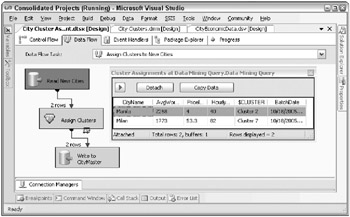
Figure 10.9: An Integration Services package to assign clusters to new cities

Implementation would also integrate this package into the rest of the nightly ETL process. The package should include the standard data and process audit functions described in Chapter 6. Ultimately, the process should be part of the package that manages the City dimension.

This nightly data mining batch process is a common one in many DW/BI systems, using a data mining model to populate a calculated field like a Default Risk score across all loan records or a Credit Rating across all customers. These scores can change depending on customer behaviors, like late payments or deposit balances . Every loan and customer may have to be rescored every night. The same batch process can be used on a one-time basis to address opportunities like identifying customers who are likely to respond to a new product offering.

Classifying Cities: Maintenance and Assessment

As the data changes, the data mining model will likely change as well. In this case, the data mining model should be re-built as data about additional cities is collected, or data about cities that have already been assigned a cluster is updated. The team would then review the resulting clusters to make sure they make sense from a business perspective. Given the nature of the business process and the changing data, this review should probably happen on a regularly scheduled basisperhaps monthly to start, then quarterly as the model and data stabilize.

This example shows how classification can be used to improve an organizations business processes. Although this dataset is too small to produce reliable results, it does generate a model that makes sense and shows how that model can be applied to new incoming data.

Case Study: Product Recommendations

The ability to recommend products that might be particularly interesting to a given customer can have a huge impact on how much your customers purchase. This example follows the data mining process from identifying the business requirements through to the implementation of a product recommendation data mining model. Its based on the Adventure Works Cycles dataset provided with SQL Server 2005. Recall from Chapter 1 that Adventure Works Cycles is a manufacturer, wholesaler, and Internet retailer of bicycles and accessories. While Microsoft has taken pains to build some interesting relationships into the data, this data may not be completely real. That is, the purchasing behaviors might not be drawn from the real world, but may in fact be made up. Data mining can help us find only relationships that are in the data.

The SQL Server data mining tutorial steps you through the process of building a model that predicts whether or not someone will be a bike buyer. While this is interesting information, it doesnt help you figure out what to display on the web page. Even if youre pretty certain someone will be a bike buyer, you dont know which bike to show them. Also, what products should you show all those folks who are not bike buyers ? Our goal in this example is to create a data mining model that produces a custom list of specific products that you can show to any given web site visitor based on demographic information you might have. To the extent that the custom product list is more appealing than a random list of products, the visitor is more likely to make a purchase.

In this example, we try to give you enough information to work through the model creation process yourself. Its not a complete step-by-step tutorial, but if youve already worked through the SQL Server data mining tutorial, you should be able to follow along and see how it works for yourself.

Product Recommendations: The Business Phase

Recall that the business phase of the data mining process involves identifying business opportunities, and building an understanding of the available data and its ability to support the data mining process. The Adventure Works Cycles data is more complete than many real-world systems weve seen, and it has more than enough customers and purchases to be interesting.

Product Recommendations: Business Opportunities

In many companies, the DW/BI team has to sell the idea of incorporating data mining into the business processes. This is usually either because the business folks dont understand the potential or because the business will have to change the transaction system, which is a big and scary task. Sometimes, the team gets lucky and data mining starts with a request from the business community. This is how it worked in the Adventure Works Cycles example. One of the folks in marketing who is responsible for e-commerce marketing came to the DW/BI team asking for ways to boost web sales. Web sales accounted for about $9,000,000 in the first half of 2004, or about one-third of Adventure Works Cycles total sales. The Marketing group has created a three-part strategy for growing the online business: Bring in more visitors (Attract), turn more visitors into customers (Convert), and develop long- term relationships with customers (Retain). The marketing person who came to the DW/BI team is responsible for the Convert strategythat is, for converting visitors to customers.

Tip 

In a case like this, if the Marketing person has a PowerPoint presentation that goes into detail on the marketing strategy, the data miner should review it. We feel sure they have such a presentation.

Because the marketing person is responsible only for conversion, the team will investigate alternatives for increasing the conversion of visitors to customers. They will check to see if the final model also increases the average dollars per sale as a beneficial side effect. After some discussion, the team decided that influencing purchasing behavior (conversion) with relevant recommendations is likely to be the best way to achieve their goals. They translated the idea of recommendations into specifics by deciding to dedicate one section of the left-hand navigation bar on the e-commerce web site to hold a list of six recommended products that will be tailored to the individual visitor. While the marketing person investigated the level of effort required to make this change on the web site, the data miner dug into the availability of relevant data.

Product Recommendations: Data Understanding

After some research, the data miner discovered that when visitors come to the Adventure Works Cycles web site, they are asked to fill out an optional demographics form (to better serve them). A few queries revealed that about two- thirds of all visitors actually do fill out the form. Because the form is a required part of the purchase process, the information is also available for all customers. In either case, this demographic information is placed in a database and in cookies in the visitor or customers browser. The DW/BI system also has all historical purchasing behavior for each customer at the individual product and line item level. Based on this investigation, the data miner felt that sufficient data was available to create a useful mining model for product recommendations.

The data miner knew from experience that behavior-based models (like purchases or page views) are generally more predictive than demographic-based models. However, there were several opportunities to make recommendations where no product-related behavioral data is available but demographic data is available. As a result, the data miner believed that two data mining models might be appropriate: one to provide recommendations on the home page and any non-product pages, and one to provide recommendations on any product- related pages. The first model would be based on demographics and would be used to predict what a visitor might be interested in given their demographic profile. The second model would be based on product interest as indicated by the product associated with each web page they visit or any products added to their cart.

At this point, the data miner wrote up a Data Mining Opportunity document to capture the goals, decisions, and approach. The overall business goal was to increase conversion rates with an ancillary goal of increasing the average dollars per sale. The strategy was to offer products that have a higher probability of being interesting to any given visitor to the web site. This strategy breaks down into two separate data mining models, one based on demographics and one based on product purchases. This decision was considered a starting point with the understanding that it would likely change during the data mining phase. This example goes through the creation of the demographics-based model. The product-based model is left as an exercise for the reader.

The team also agreed on metrics to measure the impact of the program. They would compare before and after data, looking at the change in the ratio of new customer purchases (conversions) to the total unique visitor count in the same time periods. They would also examine the change in the average shopping cart value at the time of checkout. A third impact measure would be to analyze the web logs to see how often customers viewed and clicked on a recommended link.

Product Recommendations: The Data Mining Phase

With the opportunity document as a guide, the data miner decided to begin with the demographics-based model. This section follows the development of the model from data preparation to model development and validation.

Product Recommendations: Data Preparation

The data miner decided the data source should be the AdventureWorksDW relational database. Because no web browsing data was available yet, sales data would be used to link customer demographics to product preferencesif someone actually bought something, they must have had an interest in it. The advantage of sourcing the data from the data warehouse is that it has already been through a rigorous ETL process where it was cleaned and transformed to meet basic business needs. While this is a good starting point, its often not enough for data mining.

The data miners first step was to do a little data exploration. This involved running some data profiling reports and creating some queries that examined the contents of the source tables in detail. Because the goal is to relate customer information to product information, there are two levels of granularity to the case sets. The demographic case set is generally made up of one row per observation: in this example, one row per customer. Each row has the customer key and all available demographics and other derived fields that might be useful. The product sales case set is at a lower level of detail, involving customers and the products they bought. Each row in this case set has the customer key and the product model name of the purchased product along with any other information that might be useful. Each customer case set row has a one-to-many relationship with the product sales case set (called a nested case set). You could create a single case set by joining the demographics and sales together up front and creating a denormalized table, but we prefer to rely on the data mining structure to do that for us.

After reviewing the source data in the AdventureWorksDW database, the data miner decided to pull the demographic case data from the DimCustomer table and combine it with other descriptive information from the DimGeography and DimSalesTerritory tables, and to pull the product purchasing case data from the InternetSalesFact table along with some product description fields from DimProduct and related tables. The data exploration also helped the data miner identify several additional transformations that might be useful in creating the data mining model. These are shown in Table 10.5.

Table 10.5: Additional Transformations Used to Create the Example Case Set

TRANSFORMATION	PURPOSE
Convert BirthDate to Age	Reduce the number of distinct values by moving from day to year, and provide a more meaningful value (Age) versus YearOfBirth.
Calculate YearsAsCust	DATEDIFF the DateFirstPurchase from the GetDate() to determine how many years each case has been a customer. This may help as an indicator of customer loyalty.
Create bins for YearlyIncome	Create a discrete variable called IncomeGroup to use as input to algorithms that cannot handle continuous data. Note: This is optional when creating the case set because binning can also be accomplished in the Mining Structure tab, or through the Data Mining Wizard.

As a critical part of data preparation, the data miner recognized the need to split the historical dataset into two subsets : one to train the initial model, and one to test its effectiveness. After a bit of customer count experimentation, the data miner decided to build an Integration Services package to randomly select 18,000 customers from the customer dimension and send 90 percent into the training set and the rest into the test set. The data flow shown in Figure 10.10 is the part of this package that selects the customers, adds the derived columns, splits the set into test and training datasets, and writes them out to separate tables called DMTestSet and DMTrainSet.

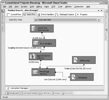
Figure 10.10: An Integration Services data flow to create test and training datasets

Tip 

This approach works for the Adventure Works Cycles customer dataset because there are only 18,484 customers total. If you have millions of customers, you might look for a more efficient way to extract training and test subsets. One possible approach is to use the last few digits of the customer key (as long as it is truly random). For example, a WHERE clause limiting the last two digits to 42 will return a 1 percent subset.

Another data flow elsewhere in this package uses the two customer sets to extract the product orders for the selected customers and write them out to a table called DMCustPurch. This is the nested product case set. Depending on how rapidly the product list changes, it might make sense to limit the datasets to only those products that have been purchased in the last year and their associated customers.

You can see the tables for the training and test datasets in the Data Source View in Figure 10.11. Figure 10.11 also includes the data model for the nested product case set.

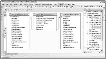
Figure 10.11: The ProductRecs datasets, presented as a data source view

The nested product case set has one or more rows for each customer. Just the fact that someone with a certain set of demographics bought a certain product is all the information you need. Notice from Figure 10.11 that the data miner decided to include some additional fields from the orders fact table that will not play a role in making recommendations but may be helpful in troubleshooting the dataset.

Tip 

Integration Services makes it easy to create physical tables snapshots of the exact datasets and relationships at a point in time. You can then use these tables to build and test many different mining models over a period of time without tainting the process with changing data. Its common to set up a separate database or even a separate server to support the data mining process and keep the production databases clear of this data mining debris.

The SQL Server 2005 Data Mining Tutorial uses views to define the case sets. This helps keep the proliferation of physical tables in the database to a minimum, but its not our preferred approach. The views need to be defined carefully ; otherwise their contents will change as the data in the underlying database is updated nightly.

At this point, the data miner has enough data in the proper form to move on to the data mining model development process.

Product Recommendations: Model Development

The data miner began the model development process by creating a new Analysis Services project in the BI Studio called ProductRecs. She added a data source that pointed to the AdventureWorksDW database and created a data source view that included the three tables created in the Integration Services package: DMTrainSet, DMTestSet, and DMCustPurch. After adding the relationships between the tables, the project and data source view looked like the screen capture shown in Figure 10.11. The keys shown in the Train and Test tables are logical primary keys assigned by the data source view.

Next , the data miner used the Data Mining Wizard to create a new mining structure by right-clicking on the Mining Structures folder and selecting New Mining Structure. The data is coming from an existing relational data warehouse, and the data miner chose the Microsoft Decision Trees data mining technique in order to predict the probability of purchasing a given product based on a set of known attributes (the demographics from the registration process). In the Specify Table Types dialog window of the wizard, the data miner checked DMTrainSet as the Case table and DMCustPurch as the Nested table.

The Specify the Training Data window can be a bit tricky because its unclear what columns should be used in what ways. For this model, all of the demographic variables will be used as input onlyyoure not trying to predict the Age or Gender of the customer with this model. Also, you need to correctly specify which DMCustPurch columns to include. At a minimum, specify a key for the nested cases.

In this example, ProductModel is the appropriate key, although its not enforced in the creation of the table. You also need to specify which column or columns to predict. Again, ProductModel is the obvious choice because it contains the description of the products to recommend. The data miner also included EnglishProductCategoryName as a predicted column because it groups the ProductModels and makes it easier to navigate later on in the Model Viewer. Finally, the data miner did not to include the quantity and amount fields because they are not relevant to this model. Remember, these are the nested purchases for each customer case. With a new visitor, youll know their demographics and can use that as input to the model, but you wont have any purchase information so it makes no sense to include it as available input data. The bottom section of the completed Specify the Training Data window is illustrated in Figure 10.12.

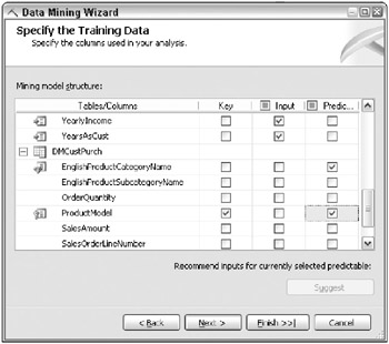
Figure 10.12: The nested table portion of the Specify the Training Data window

The next step in the Data Mining Wizard is meant to specify the content and data types of the columns in the mining structure. The data miner accepted the defaults at this point and went to the final screen, changing the mining structure name to ProductRecs1, and the mining model name to ProductRecs1-DT (for Decision Trees). After hitting the Finish button, the wizard completed the creation of the mining structure and the definition of the Decision Trees data mining model. The data miner is then able to view and verify the model definitions by viewing the Mining Models tab.

The next step is to deploy and process the model. Typically, a data miner works with one model at a time to avoid the overhead of processing all the models in the project (even though there is only one at this point, there will be more).

Tip 

To deploy and process the model, select any column in the ProductRecs1-DT model, right-click, and select Process Model. Select Yes to deploy the project, Run at the bottom of the Process Mining Model window, Close in the Process Progress window (when its finished), and finally Close back in the Process Mining Model window.

The Decision Trees algorithm generates a separate tree for each predicted value (each ProductModel), determining which variables historically have had a relationship with the purchase of that particular product. This means it will build 40 trees, one for each distinct value of the predicted variable, ProductModel, found in the DMCustPurch table.

Once the processing is complete, the data miner is finally able to explore the results. Selecting the Model Viewer tab automatically brings up the currently selected mining model in the appropriate viewerin this case, the Decision Trees sub-tab of the Microsoft Tree Viewer. The tree shown is for the first item alphabetically in the predicted results set: the tree for the All-Purpose Bike Stand, which seems to have a slight bias toward women. Selecting a more interesting product like the Mountain-200 mountain bike brings up a more interesting treeor at least one with more nodes.

The first split in the initial Mountain-200 tree is on DateFirstPurchase, and then several other fields come into play at each of the sub-branches. Immediately, the data miner recognized a problem. The DateFirstPurchase field was included in the case set inadvertently because it is an attribute of the customer dimension. However, its not a good choice for an input field for this model because visitors who have not been converted to customers will not have a DateFirstPurchase by definition. Even worse , after looking at several trees for other bicycle products, it is clear that DateFirstPurchase is also a strong splitterperhaps because the longer someone has been a customer, the more products they have purchased, and the more likely they are to have purchased a bike. A quick review of all the fields reveals that another field has the same problem: YearsAsCust. This makes sense because the field is a function of DateFirstPurchase, and contains essentially the same information. The data miner decided to remove these fields from the model and reprocess it.

One easy way to do this is to delete the fields from the Mining Structure by right-clicking on the field and selecting Delete. The more cautious way is to remove them from the ProductRecs-DT mining model by changing their type from Input to Ignore in the drop-down menu. This keeps the fields in the Mining Structure, just in case. After changing the type to Ignore on these two fields and reprocessing the model, the decision tree for the Mountain-200 now looks like the one shown in Figure 10.13.

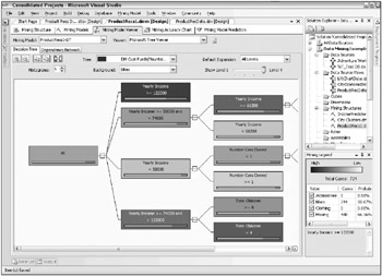
Figure 10.13: The Mountain-200 decision tree

After exploring the model in the Decision Tree tab for a bit, its useful to switch over to the Dependency Network tab. This tool provides a graphical way to see which demographic variables are predictive of which products (ProductModels). The dependency network shows the relationships between the input variables and the predicted variables. But the meaning of the initial view of the dependency network for this example, shown in Figure 10.14, is not immediately obvious. Each node in the network stands for one of the variables or products in the mining model. Some input variables are predictive of many product models, others only a few. Because we have 15 input variables and 40 individual product models and so many relationships among those variables, we end up with a spider web. In fact, the viewer automatically limits the number of nodes it will display so as not to overwhelm the user.

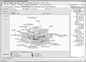
Figure 10.14: The default Dependency Network drawing for the ProductRecs1 Decision Trees model

Fortunately, theres more to the Dependency Network tab than just this view. Zooming in to see the actual names of the variables is a good way to start. Selecting a node highlights the nodes with which it has relationships. The tool uses color and arrow directions to show the nature of those relationships. Finally, the slider on the left of the pane allows the user to limit the number of relationships shown based on the strength of the relationship. The default in this viewer is to show all the relationships. Moving the slider down toward the bottom of the pane removes the weakest relationships in ascending order of strength.

WORKING WITH THE TREE VIEWER

Its worth taking a few minutes to discuss the elements of the tree viewer and how to work with it. The main pane where the picture of the tree is presented holds a lot of information. Starting with the parameter settings at the top of the Decision Tree tab in Figure 10.13 , you can see the Mountain-200 is the selected tree. (Okay, you cant really see the whole description unless you select the drop-down menu. This is an argument in favor of using very short names for your case tables and columns.) The Default Expansion parameter box to the right shows that youre viewing All Levels of the treein this case, there are four levels but only three are visible on the screen. Some trees have too many levels to display clearly so the Default Expansion control lets you limit the number of levels shown.

The tree itself is made up of several linked boxes or nodes. Each node is essentially a class with certain rules that would determine whether someone belongs in that class. (This is how decision trees can be used for classification.) The background of each node shows the proportion of the Mountain-200 cases in the node. You can change the denominator of the proportion by selecting a choice in the Background drop-down list. In Figure 10.13 , this density is relative to Bikes. Because the Mountain-200 is a bike, the background shows the number of bikes in the node divided by the number of cases in the nodein other words, the probability of someone having a Mountain-200 if they are classified in this node. The darker the node, the higher the probability that people in that node own a Mountain-200.

Selecting a node reveals the counts and probabilities for that node along with its classification rules. In Figure 10.13 , the node at the top of the second column labeled Yearly Income >= 122000 has been selected. As a result, its values and rules are displayed in the Mining Legend window in the lower right of the screen. We see that 724 cases meet the classification rules for this node. Of these 724 cases, 244 have Mountain-200 bikes, which results in a probability of 244/724 = 33.67%. In English, this reads If you are one of our customers and your income is $122,000 or greater, the chances are about 1 out of 3 that youll own a Mountain-200.

When the model is used for predicting, the theory is that probabilities based on existing customers can be applied to the folks who are not yet customers. That is, the chances are about 1 out of 3 that someone with an income of $122,000 would purchase a Mountain-200. Feed your web visitors demographic input variables into the model and it will find the nodes that the visitor classifies into and return the trees (ProductModels) that have the nodes with the highest probabilities.

 

One way to get a better sense of the relationships in the Dependency Network tab is to drag the predictive (input) variables over to one corner of the screen. Figure 10.15 shows the model from Figure 10.14 after the data miner dragged the predictive variables to the upper-right corner.

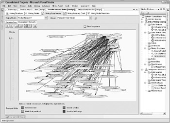
Figure 10.15: The Dependency Network with predictive variables dragged to the upper-right corner

This is still not very helpful. By zooming in on the upper-right corner, as shown in Figure 10.16, you can see that these, in fact, are the input variables. Note that there are only 14 shown in the dependency network. StateProvinceName did not play enough of a role in the model to make it onto the graph. Figure 10.16 has had another adjustment as well: The slider was moved down to about one-third of the way up from the bottom. This shows that most of the relationships, and the strongest relationships, come from only a few variables. This comes as no surprise to an experienced data miner. Often there are only a few variables that really make a differenceits just difficult to figure out ahead of time which ones theyll be.

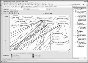
Figure 10.16: The Dependency Network zoomed in on the predictive variables

The input variables with the strongest relationships shown in Figure 10.16 are English Country Region Name, Yearly Income, and Number Cars Owned. True to the iterative data mining process, this brings up an opportunity. Removing some of the weaker variables will allow the model to explore more relationships among the stronger variables and to generate a more predictive model. For example, Figure 10.17 shows the decision tree for the Womens Mountain Shorts product based on the initial model.

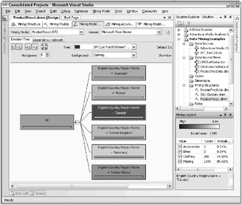
Figure 10.17: The initial decision tree for Womens Mountain Shorts

There is clearly a variation in preference for these shorts by country. About 14.5 percent of the Canadians bought a pair, but less than one-half of one percent of the Germans bought a pair. Given this information, recommending Womens Mountain Shorts to a German web site visitor is probably a waste of time.

Figure 10.18 shows the decision tree for the same product after the model has been narrowed down to five of the strongest input variables shown in Figure 10.16: Age, Yearly Income, English Country Region Name, Number of Children, and House Owner Flag.

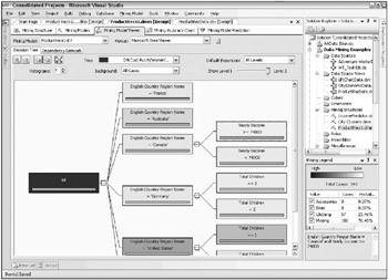
Figure 10.18: The expanded decision tree for Womens Mountain Shorts after reducing the number of input variables

The first split is still based on English Country Region Name, but now there is a second split for three of the country nodes. Canada can be split out by income, showing that Canadian customers making >= $74,000 are more likely to own a pair of Womens Mountain Shorts (probability 23.46 percent)much higher than the 15 percent we saw for Canada based on the English Country Region Name split alone in Figure 10.17.

The process of building a solid data mining model involves exploring as many iterations of the model as possible. This could mean adding variables, taking them out, combining them, adjusting the parameters of the algorithm itself, or trying one of the other algorithms that is appropriate for the problem. This is one of the strengths of the SQL Server Data Mining workbenchit is relatively easy and quick to make these changes and explore the results.

Moving back to the case study, assume that the data miner worked through several iterations and has identified the final candidate. The next step in the process is to validate the model.

Product Recommendations: Model Validation

As we described in the data mining process section, the lift chart and classification matrix in the Mining Accuracy Chart tab are designed to compare and validate models that predict single, discrete variables. The recommendations model is difficult to validate. Rather than one value per customer, the recommendations data mining model generates a probability for each ProductModel for each customer.

Another problem with validating the model is that the data miner doesnt really have historical data to test it with. The test data available, and the data used to build the model, is actually purchasing behavior, not responses to recommendations. For many data mining models, the bottom line is you wont know if it works until you try it.

Meanwhile, the data miner wants to be a bit more comfortable that the model will have a positive impact. One way to see how well the model predicts actual buying behavior is to simulate the lift chart idea in the context of recommendations. At the very least, the data miner could generate a list of the top six recommended products for each customer in the test case set and compare that list to the list of products the person actually bought. Any time a customer has purchased a product on their recommended list, the data miner would count that as a hit. This approach provides a total number of hits for the model, but it doesnt indicate if that number is a good one. You need more information: You need a baseline indication of what sales would be without the recommendations.

In order to create a baseline number for the recommendations model, the data miner also created a list of six random products for each customer in the test case set. Table 10.6 shows the results for these two tests. As it turns out, the random list isnt a realistic baseline. You wouldnt really recommend random products; you would at least use some simple data mining in the form of a query and recommend your six top-selling products to everyonepeople are more likely to want popular products. Table 10.6 includes the results for the top six list as well.

Table 10.6: Recommendations Model Validation Data Points

TEST	NUMBER OF HITS	TOTAL POSSIBLE	HIT RATE
Random Baseline	1,508	10,136	14.9%
Top Six Products	3,733	10,136	36.8%
Recommended List	4,181	10,136	41.2%

The data miner and marketing manager learn from Table 10.6 that the model is reasonably effective at predicting what customers boughtits not great, but its better than listing the top six products, and a lot better than nothing at all. Note that the hit rate in Table 10.6 has very little to do with the click-through rate youd expect to see on the web site. The real number will likely be significantly lower. However, based on these results, the data miner and the marketing manager decided to give the model a try and carefully assess its impact on the original goal of the project, increasing the percentage of visitors who become customers, and increasing the average sale amount.

Product Recommendations: The Operations Phase

The decision to go forward moved the project into the Operations phase of the data mining process. The details of the implementation are well beyond the scope of this book, but the high-level steps would involve making the data mining model available to the web server, and writing the ADOMD.NET calls to submit the visitors demographic information and to receive and post the recommendation list. Figure 10.19 shows an example of the DMX query for the ProductRecs1-DT mining model.

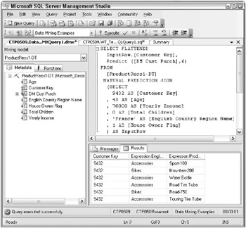
Figure 10.19: Sample DMX for a data mining query to get product recommendations based on an individuals demographics

In this case, for a 43-year-old person from France who makes $70,000 per year, has no children, and owns a house, the model recommendations include a Mountain-200 and a Road-750. This is goodyou like seeing those high-revenue bikes in the recommendations list.

Assessing the impact of the model would involve several analyses. First, the team would look at the number of unique visitors over time, and the percentage of visitors that actually become customers before and after the introduction of the recommendation list. Increasing this percentage is one of the goals of providing recommendations in the first place. This analysis would look at the average purchase amount before and after as well. It may be that the conversion rate is not significantly affected, but the average purchase amount goes up because current customers are more interested in the recommendations and end up purchasing more.

The second analysis would look at the web browsing data to see how many people click on one of the recommendation links. The analysis would follow this through to see how many people actually made a purchase. In a large enough organization, it might be worth testing the recommendation list against the top six list.

The model would also have to be maintained on a regular basis because it is built on purchasing behaviors. New product offerings and changes in fashion, preference, and price can have a big impact on the purchasing behaviorsyou dont want your recommendations to go stale.