Details

Mixed Models Theory

This section provides an overview of a likelihood -based approach to general linear mixed models. This approach simplifies and unifies many common statistical analyses, including those involving repeated measures, random effects, and random coefficients. The basic assumption is that the data are linearly related to unobserved multivariate normal random variables . Extensions to nonlinear and nonnormal situations are possible but are not discussed here. Additional theory and examples are provided in Littell et al. (1996), Verbeke and Molenberghs (1997 2000), and Brown and Prescott (1999).

Matrix Notation

Suppose that you observe n data points y ₁ ,...,y _n and that you want to explain them using n values for each of p explanatory variables x ₁₁ ,...,x _{1 p} , x ₂₁ ,...,x _{2 p} , ...,x _{n 1} ,...,x _np . The x _ij values may be either regression-type continuous variables or dummy variables indicating class membership. The standard linear model for this setup is

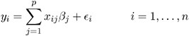
where ² ₁ ,..., ² _p are unknown fixed-effects parameters to be estimated and ₁ ,..., _n are unknown independent and identically distributed normal (Gaussian) random variables with mean 0 and variance ƒ ² .

The preceding equations can be written simultaneously using vectors and a matrix, as follows :

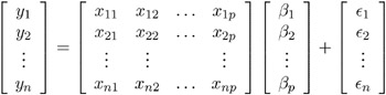
For convenience, simplicity, and extendibility, this entire system is written as

where y denotes the vector of observed y _i s, X is the known matrix of x _ij s, ² is the unknown fixed-effects parameter vector, and is the unobserved vector of independent and identically distributed Gaussian random errors.

In addition to denoting data, random variables, and explanatory variables in the preceding fashion, the subsequent development makes use of basic matrix operators such as transpose ( ² ), inverse ( ^{ˆ’ 1} ), generalized inverse ( ^ˆ’ ), determinant ( · ), and matrix multiplication. Refer to Searle (1982) for details on these and other matrix techniques.

Formulation of the Mixed Model

The previous general linear model is certainly a useful one (Searle 1971), and it is the one fitted by the GLM procedure. However, many times the distributional assumption about is too restrictive . The mixed model extends the general linear model by allowing a more flexible specification of the covariance matrix of . In other words, it allows for both correlation and heterogeneous variances, although you still assume normality.

The mixed model is written as

where everything is the same as in the general linear model except for the addition of the known design matrix, Z , and the vector of unknown random-effects parameters, ³ . The matrix Z can contain either continuous or dummy variables, just like X . The name mixed model comes from the fact that the model contains both fixed-effects parameters, ² , and random-effects parameters, ³ . Refer to Henderson (1990) and Searle, Casella, and McCulloch (1992) for historical developments of the mixed model.

A key assumption in the foregoing analysis is that ³ and are normally distributed with

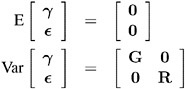
The variance of y is, therefore, V = ZGZ ² + R . You can model V by setting up the random-effects design matrix Z and by specifying covariance structures for G and R .

Note that this is a general specification of the mixed model, in contrast to many texts and articles that discuss only simple random effects. Simple random effects are a special case of the general specification with Z containing dummy variables, G containing variance components in a diagonal structure, and R = ƒ ² I _n , where I _n denotes the n — n identity matrix. The general linear model is a further special case with Z = and R = ƒ ² I _n .

The following two examples illustrate the most common formulations of the general linear mixed model.

Example: Growth Curve with Compound Symmetry

Suppose that you have three growth curve measurements for s individuals and that you want to fit an overall linear trend in time. Your X matrix is as follows:

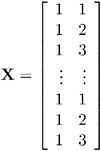
The first column (coded entirely with 1s) fits an intercept, and the second column (coded with times of 1 , 2 , 3) fits a slope. Here, n =3 s and p =2.

Suppose further that you want to introduce a common correlation among the observations from a single individual, with correlation being the same for all individuals. One way of setting this up in the general mixed model is to eliminate the Z and G matrices and let the R matrix be block diagonal with blocks corresponding to the individuals and with each block having the compound-symmetry structure. This structure has two unknown parameters, one modeling a common covariance and the other a residual variance. The form for R would then be as follows:

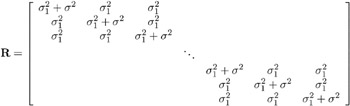
where blanks denote zeroes. There are 3 s rows and columns altogether, and the common correlation is .

The PROC MIXED code to fit this model is as follows:

  proc mixed;   class indiv;   model y = time;   repeated / type=cs subject=indiv;   run;  

Here, indiv is a classification variable indexing individuals. The MODEL statement fits a straight line for time ; the intercept is fit by default just as in PROC GLM. The REPEATED statement models the R matrix: TYPE=CS specifies the compound symmetry structure, and SUBJECT=INDIV specifies the blocks of R .

An alternative way of specifying the common intra-individual correlation is to let

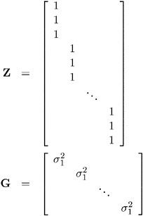
and R = ƒ ² I _n . The Z matrix has 3 s rows and s columns, and G is s — s .

You can set up this model in PROC MIXED in two different but equivalent ways:

  proc mixed;   class indiv;   model y = time;   random indiv;   run;   proc mixed;   class indiv;   model y = time;   random intercept / subject=indiv;   run;  

Both of these specifications fit the same model as the previous one that used the REPEATED statement; however, the RANDOM specifications constrain the correlation to be positive whereas the REPEATED specification leaves the correlation unconstrained.

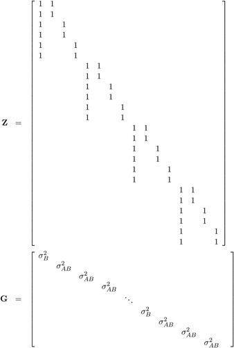
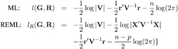
Example: Split-Plot Design

• The split-plot design involves two experimental treatment factors, A and B , and two different sizes of experimental units to which they are applied (refer to Winer 1971, Snedecor and Cochran 1980, Milliken and Johnson 1992, and Steel, Torrie, and Dickey 1997). The levels of A are randomly assigned to the larger sized experimental unit, called whole plots , whereas the levels of B are assigned to the smaller sized experimental unit, the subplots . The subplots are assumed to be nested within the whole plots, so that a whole plot consists of a cluster of subplots and a level of A is applied to the entire cluster.

• Such an arrangement is often necessary by nature of the experiment, the classical example being the application of fertilizer to large plots of land and different crop varieties planted in subdivisions of the large plots. For this example, fertilizer is the whole plot factor A and variety is the subplot factor B .

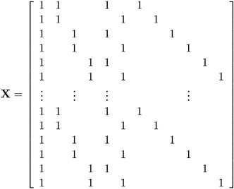
• The first example is a split-plot design for which the whole plots are arranged in a randomized block design. The appropriate PROC MIXED code is as follows:

    proc mixed;   class a b block;   model y = ab;   random block a*block;   run;  

  Here

  

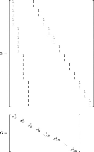
• and X , Z , and G have the following form:

  
  

• where is the variance component for Block and is the variance component for A * Block . Changing the RANDOM statement to

    random int a / subject=block;  

• fits the same model, but with Z and G sorted differently.

Estimating G and R in the Mixed Model

Estimation is more difficult in the mixed model than in the general linear model. Not only do you have ² as in the general linear model, but you have unknown parameters in ³ , G , and R as well. Least squares is no longer the best method. Generalized least squares (GLS) is more appropriate, minimizing

However, it requires knowledge of V and, therefore, knowledge of G and R . Lacking such information, one approach is to use estimated GLS, in which you insert some reasonable estimate for V into the minimization problem. The goal thus becomes finding a reasonable estimate of G and R .

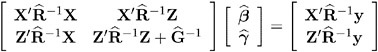
In many situations, the best approach is to use likelihood-based methods , exploiting the assumption that ³ and are normally distributed (Hartley and Rao 1967; Patterson and Thompson 1971; Harville 1977; Laird and Ware 1982; Jennrich and Schluchter 1986). PROC MIXED implements two likelihood-based methods: maximum likelihood (ML) and restricted/residual maximum likelihood (REML). A favorable theoretical property of ML and REML is that they accommodate data that are missing at random (Rubin 1976; Little 1995).

PROC MIXED constructs an objective function associated with ML or REML and maximizes it over all unknown parameters. Using calculus, it is possible to reduce this maximization problem to one over only the parameters in G and R . The corresponding log-likelihood functions are as follows:

where r = y ˆ’ X ( X ² V ^{ˆ’ 1} X ) ˆ’ X ² V ^{ˆ’ 1} y and p is the rank of X . PROC MIXED actually minimizes ˆ’ 2 times these functions using a ridge-stabilized Newton-Raphson algorithm. Lindstrom and Bates (1988) provide reasons for preferring Newton-Raphson to the Expectation-Maximum (EM) algorithm described in Dempster, Laird, and Rubin (1977) and Laird, Lange, and Stram (1987), as well as analytical details for implementing a QR-decomposition approach to the problem. Wolfinger, Tobias, and Sall (1994) present the sweep-based algorithms that are implemented in PROC MIXED.

One advantage of using the Newton-Raphson algorithm is that the second derivative matrix of the objective function evaluated at the optima is available upon completion. Denoting this matrix H , the asymptotic theory of maximum likelihood (refer to Serfling 1980) shows that 2 H ˆ’ ¹ is an asymptotic variance-covariance matrix of the estimated parameters of G and R . Thus, tests and confidence intervals based on asymptotic normality can be obtained. However, these can be unreliable in small samples, especially for parameters such as variance components which have sampling distributions that tend to be skewed to the right.

If a residual variance ƒ ² is a part of your mixed model, it can usually be profiled out of the likelihood. This means solving analytically for the optimal ƒ ² and plugging this expression back into the likelihood formula (refer to Wolfinger, Tobias, and Sall 1994). This reduces the number of optimization parameters by one and can improve convergence properties. PROC MIXED profiles the residual variance out of the log likelihood whenever it appears reasonable to do so. This includes the case when R equals ƒ ² I and when it has blocks with a compound symmetry, time series, or spatial structure. PROC MIXED does not profile the log likelihood when R has unstructured blocks, when you use the HOLD= or NOITER option in the PARMS statement, or when you use the NOPROFILE option in the PROC MIXED statement.

Instead of ML or REML, you can use the noniterative MIVQUE0 method to estimate G and R (Rao 1972; LaMotte 1973; Wolfinger, Tobias, and Sall 1994). In fact, by default PROC MIXED uses MIVQUE0 estimates as starting values for the ML and REML procedures. For variance component models, another estimation method involves equating Type I, II, or III expected mean squares to their observed values and solving the resulting system. However, Swallow and Monahan (1984) present simulation evidence favoring REML and ML over MIVQUE0 and other method-of-moment estimators.

Estimating ² and ³ in the Mixed Model

ML, REML, MIVQUE0, or Type1 “Type3 provide estimates of G and R , which are denoted and , respectively. To obtain estimates of ² and ³ , the standard method is to solve the mixed model equations (Henderson 1984):

The solutions can also be written as

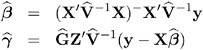
and have connections with empirical Bayes estimators (Laird and Ware 1982, Carlin and Louis 1996).

Note that the mixed model equations are extended normal equations and that the preceding expression assumes that is nonsingular. For the extreme case when the eigenvalues of are very large, ^{ˆ’ 1} contributes very little to the equations and is close to what it would be if ³ actually contained fixed-effects parameters. On the other hand, when the eigenvalues of are very small, ^{ˆ’ 1} dominates the equations and is close to 0. For intermediate cases, ^{ˆ’ 1} can be viewed as shrinking the fixed-effects estimates of ³ towards 0 (Robinson 1991).

If is singular, then the mixed model equations are modified (Henderson 1984) as follows:

where is the lower- triangular Cholesky root of , satisfying = ² . Both and a generalized inverse of the left-hand-side coefficient matrix are then transformed using to determine .

An example of when the singular form of the equations is necessary is when a variance component estimate falls on the boundary constraint of 0.

Model Selection

The previous section on estimation assumes the specification of a mixed model in terms of X , Z , G , and R . Even though X and Z have known elements, their specific form and construction is flexible, and several possibilities may present themselves for a particular data set. Likewise, several different covariance structures for G and R might be reasonable.

Space does not permit a thorough discussion of model selection, but a few brief comments and references are in order. First, subject matter considerations and objectives are of great importance when selecting a model; refer to Diggle (1988) and Lindsey (1993).

Second, when the data themselves are looked to for guidance, many of the graphical methods and diagnostics appropriate for the general linear model extend to the mixed model setting as well (Christensen, Pearson, and Johnson 1992).

Finally, a likelihood-based approach to the mixed model provides several statistical measures for model adequacy as well. The most common of these are the likelihood ratio test and Akaike s and Schwarz s criteria (Bozdogan 1987; Wolfinger 1993, Keselman et al. 1998, 1999).

Statistical Properties

If G and R are known, is the best linear unbiased estimator (BLUE) of ² , and is the best linear unbiased predictor (BLUP) of ³ (Searle 1971; Harville 1988, 1990; Robinson 1991; McLean, Sanders, and Stroup 1991). Here, best means minimum mean squared error. The covariance matrix of ( ˆ’ ² , ˆ’ ³ ) is

where ^ˆ’ denotes a generalized inverse (refer to Searle 1971).

However, G and R are usually unknown and are estimated using one of the aforementioned methods. These estimates, and , are therefore simply substituted into the preceding expression to obtain

as the approximate variance-covariance matrix of ( ˆ’ ² ˆ’ ³ ). In this case, the BLUE and BLUP acronyms no longer apply, but the word empirical is often added to indicate such an approximation . The appropriate acronyms thus become EBLUE and EBLUP.

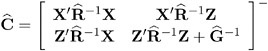
McLean and Sanders (1988) show that can also be written as

where

Note that ₁₁ is the familiar estimated generalized least-squares formula for the variance-covariance matrix of .

As a cautionary note, tends to underestimate the true sampling variability of ( ) because no account is made for the uncertainty in estimating G and R . Although inflation factors have been proposed (Kackar and Harville 1984; Kass and Steffey 1989; Prasad and Rao 1990), they tend to be small for data sets that are fairly well balanced. PROC MIXED does not compute any inflation factors by default, but rather accounts for the downward bias by using the approximate t and F statistics described subsequently. The DDFM=KENWARDROGER option in the MODEL statement prompts PROC MIXED to compute a specificinflation factor along with Satterthwaite-based degrees of freedom.

Inference and Test Statistics

For inferences concerning the covariance parameters in your model, you can use likelihood-based statistics. One common likelihood-based statistic is the Wald Z , which is computed as the parameter estimate divided by its asymptotic standard error. The asymptotic standard errors are computed from the inverse of the second derivative matrix of the likelihood with respect to each of the covariance parameters. The Wald Z is valid for large samples, but it can be unreliable for small data sets and for parameters such as variance components, which are known to have a skewed or bounded sampling distribution.

A better alternative is the likelihood ratio ² . This statistic compares two covariance models, one a special case of the other. To compute it, you must run PROC MIXED twice, once for each of the two models, and then subtract the corresponding values of ˆ’ 2 times the log likelihoods. You can use either ML or REML to construct this statistic, which tests whether the full model is necessary beyond the reduced model.

As long as the reduced model does not occur on the boundary of the covariance parameter space, the ² statistic computed in this fashion has a large-sample sampling distribution that is ² with degrees of freedom equal to the difference in the number of covariance parameters between the two models. If the reduced model does occur on the boundary of the covariance parameter space, the asymptotic distribution becomes a mixture of ² distributions (Self and Liang 1987). A common example of this is when you are testing that a variance component equals its lower boundary constraint of 0.

A final possibility for obtaining inferences concerning the covariance parameters is to simulate or resample data from your model and construct empirical sampling distributions of the parameters. The SAS macro language and the ODS system are useful tools in this regard.

For inferences concerning the fixed- and random-effects parameters in the mixed model, consider estimable linear combinations of the following form:

The estimability requirement (Searle 1971) applies only to the ² -portion of L , as any linear combination of ³ is estimable. Such a formulation in terms of a general L matrix encompasses a wide variety of common inferential procedures such as those employed with Type I “Type III tests and LS-means. The CONTRAST and ESTIMATE statements in PROC MIXED enable you to specify your own L matrices. Typically, inference on fixed-effects is the focus, and, in this case, the ³ -portion of L is assumed to contain all 0s.

Statistical inferences are obtained by testing the hypothesis

or by constructing point and interval estimates.

When L consists of a single row, a general t -statistic can be constructed as follows (refer to McLean and Sanders 1988, Stroup 1989a):

Under the assumed normality of ³ and , t has an exact t -distribution only for data exhibiting certain types of balance and for some special unbalanced cases. In general, t is only approximately t -distributed, and its degrees of freedom must be estimated. See the DDFM= option on page 2693 for a description of the various degrees-of-freedom methods available in PROC MIXED.

With being the approximate degrees of freedom, the associated confidence interval is

where t is the (1 ˆ’ ± / 2)100th percentile of the .

When the rank of L is greater than 1, PROC MIXED constructs the following general F -statistic:

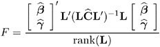
Analogous to t , F in general has an approximate F -distribution with rank( L ) numerator degrees of freedom and denominator degrees of freedom.

The t -and F -statistics enable you to make inferences about your fixed effects, which account for the variance-covariance model you select. An alternative is the ² statistic associated with the likelihood ratio test. This statistic compares two fixed-effects models, one a special case of the other. It is computed just as when comparing different covariance models, although you should use ML and not REML here because the penalty term associated with restricted likelihoods depends upon the fixed-effects specification.

Parameterization of Mixed Models

Recall that a mixed model is of the form

where y represents univariate data, ² is an unknown vector of fixed effects with known model matrix X , ³ is an unknown vector of random effects with known model matrix Z , and is an unknown random error vector.

PROC MIXED constructs a mixed model according to the specifications in the MODEL, RANDOM, and REPEATED statements. Each effect in the MODEL statement generates one or more columns in the model matrix X , and each effect in the RANDOM statement generates one or more columns in the model matrix Z . Effects in the REPEATED statement do not generate model matrices; they serve only to index observations within subjects. This section shows precisely how PROC MIXED builds X and Z .

Intercept

By default, all models automatically include a column of 1s in X to estimate a fixed-effect intercept parameter ¼ . You can use the NOINT option in the MODEL statement to suppress this intercept. The NOINT option is useful when you are specifying a classification effect in the MODEL statement and you want the parameter estimate to be in terms of the mean response for each level of that effect, rather than in terms of a deviation from an overall mean.

By contrast, the intercept is not included by default in Z . To obtain a column of 1s in Z , you must specify in the RANDOM statement either the INTERCEPT effect or some effect that has only one level.

Regression Effects

Numeric variables, or polynomial terms involving them, may be included in the model as regression effects (covariates). The actual values of such terms are included as columns of the model matrices X and Z . You can use the bar operator with a regression effect to generate polynomial effects. For instance, XXX expands to X X*X X*X*X, a cubic model.

Main Effects

If a class variable has m levels, PROC MIXED generates m columns in the model matrix for its main effect. Each column is an indicator variable for a given level. The order of the columns is the sort order of the values of their levels and can be controlled with the ORDER= option in the PROC MIXED statement. The following table is an example.

Data		I	A		B
A	B	¼	A1	A2	B1	B2	B3
1	1	1	1		1
1	2	1	1			1
1	3	1	1				1
2	1	1		1	1
2	2	1		1		1
2	3	1		1			1

Typically, there are more columns for these effects than there are degrees of freedom for them. In other words, PROC MIXED uses an over-parameterized model.

Interaction Effects

Often a model includes interaction (crossed) effects. With an interaction, PROC MIXED first reorders the terms to correspond to the order of the variables in the CLASS statement. Thus, B * A becomes A * B if A precedes B in the CLASS statement. Then, PROC MIXED generates columns for all combinations of levels that occur in the data. The order of the columns is such that the rightmost variables in the cross index faster than the leftmost variables. Empty columns (that would contain all 0s) are not generated for X , but they are for Z .

Data		I	A		B			A * B
A	B	¼	A1	A2	B1	B2	B3	A1B1	A1B2	A1B3	A2B1	A2B2	A2B3
1	1	1	1		1			1
1	2	1	1			1			1
1	3	1	1				1			1
2	1	1		1	1						1
2	2	1		1		1						1
2	3	1		1			1						1

In the preceding matrix, main-effects columns are not linearly independent of crossed-effect columns; in fact, the column space for the crossed effects contains the space of the main effect.

When your model contains many interaction effects, you may be able to code them more parsimoniously using the bar operator ( ). The bar operator generates all possible interaction effects. For example, A B C expands to ABA * BCA * CB * C A * B * C . To eliminate higher-order interaction effects, use the at sign ( @ ) in conjunction with the bar operator. For instance, A B C D @2 expands to ABA * BC A * CB * CDA * DB * DC * D .

Nested Effects

Nested effects are generated in the same manner as crossed effects. Hence, the design columns generated by the following two statements are the same (but the ordering of the columns is different):

  model Y=A B(A);   model Y=A A*B;  

The nesting operator in PROC MIXED is more a notational convenience than an operation distinct from crossing . Nested effects are typically characterized by the property that the nested variables never appear as main effects. The order of the variables within nesting parentheses is made to correspond to the order of these variables in the CLASS statement. The order of the columns is such that variables outside the parentheses index faster than those inside the parentheses, and the rightmost nested variables index faster than the leftmost variables.

Data		I	A		B ( A )
A	B	¼	A1	A2	B1A1	B2A1	B3A1	B1A2	B2A2	B3A2
1	1	1	1		1
1	2	1	1			1
1	3	1	1				1
2	1	1		1				1
2	2	1		1					1
2	3	1		1						1

Note that nested effects are often distinguished from interaction effects by the implied randomization structure of the design. That is, they usually indicate random effects within a fixed-effects framework. The fact that random effects can be modeled directly in the RANDOM statement may make the specification of nested effects in the MODEL statement unnecessary.

Continuous-Nesting-Class Effects

When a continuous variable nests with a class variable, the design columns are constructed by multiplying the continuous values into the design columns for the class effect.

Data		I	A		X ( A )
X	A	¼	A1	A2	X(A1)	X(A2)
21	1	1	1		21
24	1	1	1		24
22	1	1	1		22
28	2	1		1		28
19	2	1		1		19
23	2	1		1		23

This model estimates a separate slope for X within each level of A .

Continuous-by-Class Effects

Continuous-by-class effects generate the same design columns as continuous-nesting-class effects. The two models are made different by the presence of the continuous variable as a regressor by itself, as well as a contributor to a compound effect.

Data		I	X	A		X * A
X	A	¼	X	A1	A2	X*A1	X*A2
21	1	1	21	1		21
24	1	1	24	1		24
22	1	1	22	1		22
28	2	1	28		1		28
19	2	1	19		1		19
23	2	1	23		1		23

You can use continuous-by-class effects to test for homogeneity of slopes.

General Effects

An example that combines all the effects is X1 * X2 * A * B * C ( DE ). The continuous list comes first, followed by the crossed list, followed by the nested list in parentheses. You should be aware of the sequencing of parameters when you use the CONTRAST or ESTIMATE statements to compute some function of the parameter estimates.

Effects may be renamed by PROC MIXED to correspond to ordering rules. For example, B * A ( ED ) may be renamed A * B ( DE ) to satisfy the following:

• Class variables that occur outside parentheses (crossed effects) are sorted in the order in which they appear in the CLASS statement.

• Variables within parentheses (nested effects) are sorted in the order in which they appear in the CLASS statement.

The sequencing of the parameters generated by an effect can be described by which variables have their levels indexed faster:

• Variables in the crossed list index faster than variables in the nested list.

• Within a crossed or nested list, variables to the right index faster than variables to the left.

For example, suppose a model includes four effects ” A , B , C , and D ”each having two levels, 1 and 2. If the CLASS statement is

  class A B C D;  

then the order of the parameters for the effect B*A(C D), which is renamed A * B ( CD ), is

A 1 B 1 C 1 D 1	’	A 1 B 2 C 1 D 1	’	A 2 B 1 C 1 D 1	’	A 2 B 2 C 1 D 1	’
A 1 B 1 C 1 D 2	’	A 1 B 2 C 1 D 2	’	A 2 B 1 C 1 D 2	’	A 2 B 2 C 1 D 2	’
A 1 B 1 C 2 D 1	’	A 1 B 2 C 2 D 1	’	A 2 B 1 C 2 D 1	’	A 2 B 2 C 2 D 1	’
A 1 B 1 C 2 D 2	’	A 1 B 2 C 2 D 2	’	A 2 B 1 C 2 D 2	’	A 2 B 2 C 2 D 2

Note that first the crossed effects B and A are sorted in the order in which they appear in the CLASS statement so that A precedes B in the parameter list. Then, for each combination of the nested effects in turn , combinations of A and B appear. The B effect moves fastest because it is rightmost in the cross list. Then A moves next fastest, and D moves next fastest. The C effect is the slowest since it is leftmost in the nested list.

When numeric levels are used, levels are sorted by their character format, which may not correspond to their numeric sort sequence (for example, noninteger levels). Therefore, it is advisable to include a desired format for numeric levels or to use the ORDER=INTERNAL option in the PROC MIXED statement to ensure that levels are sorted by their internal values.

Implications of the Non-Full-Rank Parameterization

For models with fixed-effects involving class variables, there are more design columns in X constructed than there are degrees of freedom for the effect. Thus, there are linear dependencies among the columns of X . In this event, all of the parameters are not estimable; there is an infinite number of solutions to the mixed model equations. PROC MIXED uses a generalized (g2) inverse to obtain values for the estimates (Searle 1971). The solution values are not displayed unless you specify the SOLUTION option in the MODEL statement. The solution has the characteristic that estimates are 0 whenever the design column for that parameter is a linear combination of previous columns. With this parameterization, hypothesis tests are constructed to test linear functions of the parameters that are estimable.

Some procedures (such as the CATMOD procedure) reparameterize models to full rank using restrictions on the parameters. PROC GLM and PROC MIXED do not reparameterize, making the hypotheses that are commonly tested more understandable. Refer to Goodnight (1978) for additional reasons for not reparameterizing.

Missing Level Combinations

PROC MIXED handles missing level combinations of classification variables similarly to the way PROC GLM does. Both procedures delete fixed-effects parameters corresponding to missing levels in order to preserve estimability. However, PROC MIXED does not delete missing level combinations for random-effects parameters because linear combinations of the random-effects parameters are always estimable. These conventions can affect the way you specify your CONTRAST and ESTIMATE coefficients.

Default Output

The following sections describe the output PROC MIXED produces by default. This output is organized into various tables, and they are discussed in order of appearance.

Model Information

The Model Information table describes the model, some of the variables it involves, and the method used in fitting it. It also lists the method (profile, fit, factor, or none) for handling the residual variance in the model. The profile method concentrates the residual variance out of the optimization problem, whereas the fit method retains it as a parameter in the optimization. The factor method keeps the residual fixed, and none is displayed when a residual variance is not a part of the model.

The Model Information table also has a row labeled Fixed Effects SE Method. This row describes the method used to compute the approximate standard errors for the fixed-effects parameter estimates and related functions of them. The two possibilities for this row are Model-Based, which is the default method, and Empirical, which results from using the EMPIRICAL option in the PROC MIXED statement.

For ODS purposes, the label of the Model Information table is ModelInfo.

Class Level Information

The Class Level Information table lists the levels of every variable specified in the CLASS statement. You should check this information to make sure the data are correct. You can adjust the order of the CLASS variable levels with the ORDER= option in the PROC MIXED statement. For ODS purposes, the label of the Class Level Information table is ClassLevels.

Dimensions

The Dimensions table lists the sizes of relevant matrices. This table can be useful in determining CPU time and memory requirements. For ODS purposes, the label of the Dimensions table is Dimensions.

Number of Observations

The Number of Observations table shows the number of observations read from the data set and the number of observations used in fitting the model.

Iteration History

The Iteration History table describes the optimization of the residual log likelihood or log likelihood described on page 2738. The function to be minimized (the objective function ) is ˆ’ 2 l for ML and ˆ’ 2 l _R for REML; the column name of the objective function in the Iteration History table is -2 Log Like for ML and -2 Res Log Like for REML. The minimization is performed using a ridge-stabilized Newton-Raphson algorithm, and the rows of this table describe the iterations that this algorithm takes in order to minimize the objective function.

The Evaluations column of the Iteration History table tells how many times the objective function is evaluated during each iteration.

The Criterion column of the Iteration History table is, by default, a relative Hessian convergence quantity given by

where f _k is the value of the objective function at iteration k , g _k is the gradient (first derivative) of f _k , and H _k is the Hessian (second derivative) of f _k . If H _k is singular, then PROC MIXED uses the following relative quantity:

To prevent the division by f _k , use the ABSOLUTE option in the PROC MIXED statement. To use a relative function or gradient criterion, use the CONVF or CONVG options, respectively.

The Hessian criterion is considered superior to function and gradient criteria because it measures orthogonality rather than lack of progress (Bates and Watts 1988). Provided the initial estimate is feasible and the maximum number of iterations is not exceeded, the Newton-Raphson algorithm is considered to have converged when the criterion is less than the tolerance specified with the CONVF, CONVG, or CONVH option in the PROC MIXED statement. The default tolerance is 1E ˆ’ 8. If convergence is not achieved, PROC MIXED displays the estimates of the parameters at the last iteration.

A convergence criterion that is missing indicates that a boundary constraint has been dropped; it is usually not a cause for concern.

If you specify the ITDETAILS option in the PROC MIXED statement, then the covariance parameter estimates at each iteration are included as additional columns in the Iteration History table.

For ODS purposes, the label of the Iteration History table is IterHistory.

Covariance Parameter Estimates

The Covariance Parameter Estimates table contains the estimates of the parameters in G and R (see the Estimating G and R in the Mixed Model section on page 2737). Their values are labeled in the Cov Parm table along with Subject and Group information if applicable . The estimates are displayed in the Estimate column and are the results of one of the following estimation methods: REML, ML, MIVQUE0, SSCP, Type1, Type2, or Type3.

If you specify the RATIO option in the PROC MIXED statement, the Ratio column is added to the table listing the ratios of each parameter estimate to that of the residual variance.

Requesting the COVTEST option in the PROC MIXED statement produces the Std Error, Z Value, and Pr Z columns. The Std Error column contains the approximate standard errors of the covariance parameter estimates. These are the square roots of the diagonal elements of the observed inverse Fisher information matrix, which equals 2 H ^{ˆ’ 1} , where H is the Hessian matrix. The H matrix consists of the second derivatives of the objective function with respect to the covariance parameters; refer to Wolfinger, Tobias, and Sall (1994) for formulas. When you use the SCORING= option and PROC MIXED converges without stopping the scoring algorithm, PROC MIXED uses the expected Hessian matrix to compute the covariance matrix instead of the observed Hessian. The observed or expected inverse Fisher information matrix can be viewed as an asymptotic covariance matrix of the estimates.

The Z Value column is the estimate divided by its approximate standard error, and the Pr Z column is the one- or two-tailed area of the standard Gaussian density outside of the Z -value. The MIXED procedure computes one-sided p-values for the residual variance and for covariance parameters with a lower bound of 0. The procedure computes two-sided p-values otherwise . These statistics constitute Wald tests of the covariance parameters, and they are valid only asymptotically.

Caution: Wald tests can be unreliable in small samples.

For ODS purposes, the label of the Covariance Parameter Estimates table is CovParms.

Fit Statistics

The Fit Statistics table provides some statistics about the estimated mixed model. Expressions for the ˆ’ 2 times the log likelihood are provided in the Estimating G and RintheMixedModel section on page 2737. If the log likelihood is an extremely large number, then PROC MIXED has deemed the estimated V matrix to be singular. In this case, all subsequent results should be viewed with caution.

In addition, the Fit Statistics table lists three information criteria: AIC, AICC, and BIC, all in smaller-is-better form. Expressions for these criteria are described under the IC option on page 2676.

For ODS purposes, the label of the Model Fitting Information table is FitStatistics.

Null Model Likelihood Ratio Test

If one covariance model is a submodel of another, you can carry out a likelihood ratio test for the significance of the more general model by computing ˆ’ 2 times the difference between their log likelihoods. Then compare this statistic to the ² distribution with degrees of freedom equal to the difference in the number of parameters for the two models.

This test is reported in the Null Model Likelihood Ratio Test table to determine whether it is necessary to model the covariance structure of the data at all. The ChiSquare value is ˆ’ 2 times the log likelihood from the null model minus ˆ’ 2 times the log likelihood from the fitted model, where the null model is the one with only the fixed effects listed in the MODEL statement and R = ƒ ² I . This statistic has an asymptotic ² -distribution with q ˆ’ 1 degrees of freedom, where q is the effective number of covariance parameters (those not estimated to be on a boundary constraint). The Pr > ChiSq column contains the upper-tail area from this distribution. This p -value can be used to assess the significance of the model fit.

This test is not produced for cases where the null hypothesis lies on the boundary of the parameter space, which is typically for variance component models. This is because the standard asymptotic theory does not apply in this case (Self and Liang 1987, Case 5).

If you specify a PARMS statement, PROC MIXED constructs a likelihood ratio test between the best model from the grid search and the final fitted model and reports the results in the Parameter Search table.

For ODS purposes, the label of the Null Model Likelihood Ratio Test table is LRT.

Type 3 Tests of Fixed Effects

The Type 3 Tests of Fixed Effects table contains hypothesis tests for the significance of each of the fixed effects, that is, those effects you specify in the MODEL statement. By default, PROC MIXED computes these tests by first constructing a Type III L matrix (see Chapter 11, The Four Types of Estimable Functions, ) for each effect. This L matrix is then used to compute the following F -statistic:

A p -value for the test is computed as the tail area beyond this statistic from an F -distribution with NDF and DDF degrees of freedom. The numerator degrees of freedom (NDF) is the row rank of L , and the denominator degrees of freedom is computed using one of the methods described under the DDFM= option on page 2693. Small values of the p -value (typically less than 0.05 or 0.01) indicate a significant effect.

You can use the HTYPE= option in the MODEL statement to obtain tables of Type I (sequential) tests and Type II (adjusted) tests in addition to or instead of the table of Type III (partial) tests.

You can use the CHISQ option in the MODEL statement to obtain Wald ² tests of the fixed effects. These are carried out by using the numerator of the F -statistic and comparing it with the ² distribution with NDF degrees of freedom. It is more liberal than the F -test because it effectively assumes an infinite denominator degrees of freedom.

For ODS purposes, the label of the Type 1 Tests of Fixed Effects through the Type 3 Tests of Fixed Effects tables are Tests1 through Tests3, respectively.

ODS Table Names

Each table created by PROC MIXED has a name associated with it, and you must use this name to reference the table when using ODS statements. These names are listed in Table 46.8.

Table 46.8: ODS Tables Produced in PROC MIXED

Table Name	Description	Required Statement / Option
AccRates	acceptance rates for posterior sampling	PRIOR
AsyCorr	asymptotic correlation matrix of covariance parameters	PROC MIXED ASYCORR
AsyCov	asymptotic covariance matrix of covariance parameters	PROC MIXED ASYCOV
Base	base densities used for posterior sampling	PRIOR
Bound	computed bound for posterior rejection sampling	PRIOR
CholG	Cholesky root of the estimated G matrix	RANDOM / GC
CholR	Cholesky root of blocks of the estimated R matrix	REPEATED / RC
CholV	Cholesky root of blocks of the estimated V matrix	RANDOM / VC
ClassLevels	level information from the CLASS statement	default output
Coef	L matrix coefficients	E option on MODEL, CONTRAST, ESTIMATE, or LSMEANS
Contrasts	results from the CONTRAST statements	CONTRAST
ConvergenceStatus	convergence status	default
CorrB	approximate correlation matrix of fixed-effects parameter estimates	MODEL / CORRB
CovB	approximate covariance matrix of fixed-effects parameter estimates	MODEL / COVB
CovParms	estimated covariance parameters	default output
Diffs	differences of LS-means	LSMEANS / DIFF (or PDIFF)
Dimensions	dimensions of the model	default output
Estimates	results from ESTIMATE statements	ESTIMATE
FitStatistics	fit statistics	default
G	estimated G matrix	RANDOM / G
GCorr	correlation matrix from the estimated G matrix	RANDOM / GCORR
HLM1	Type 1 Hotelling-Lawley-McKeon tests of fixed effects	MODEL / HTYPE=1 and REPEATED / HLM TYPE=UN
HLM2	Type 2 Hotelling-Lawley-McKeon tests of fixed effects	MODEL / HTYPE=2 and REPEATED / HLM TYPE=UN
HLM3	Type 3 Hotelling-Lawley-McKeon tests of fixed effects	REPEATED / HLM TYPE=UN
HLPS1	Type 1 Hotelling-Lawley-Pillai-Samson tests of fixed effects	MODEL / HTYPE=1 and REPEATED / HLPS TYPE=UN
HLPS2	Type 2 Hotelling-Lawley-Pillai-Samson tests of fixed effects	MODEL / HTYPE=1 and REPEATED / HLPS TYPE=UN
HLPS3	Type 3 Hotelling-Lawley-Pillai-Samson tests of fixed effects	REPEATED / HLPS TYPE=UN
Influence	influence diagnostics	MODEL / INFLUENCE
InfoCrit	information criteria	PROC MIXED IC
InvCholG	inverse Cholesky root of the estimated G matrix	RANDOM / GCI
InvCholR	inverse Cholesky root of blocks of the estimated R matrix	REPEATED / RCI
InvCholV	inverse Cholesky root of blocks of the estimated V matrix	RANDOM / VCI
InvCovB	inverse of approximate covariance matrix of fixed-effects parameter estimates	MODEL / COVBI
InvG	inverse of the estimated G matrix	RANDOM / GI
InvR	inverse of blocks of the estimated R matrix	REPEATED / RI
InvV	inverse of blocks of the estimated V matrix	RANDOM / VI
IterHistory	iteration history	default output
LComponents	single degree of freedom estimates corresponding to rows of the L matrix for fixed effects	MODEL / LCOMPONENTS
LRT	likelihood ratio test	default output
LSMeans	LS-means	LSMEANS
MMEq	mixed model equations	PROC MIXED MMEQ
MMEqSol	mixed model equations solution	PROC MIXED MMEQSOL
ModelInfo	model information	default output
NObs	number of observations read and used	default output
ParmSearch	parameter search values	PARMS
Posterior	posterior sampling information	PRIOR
R	blocks of the estimated R matrix	REPEATED / R
RCorr	correlation matrix from blocks of the estimated R matrix	REPEATED / RCORR
Search	posterior density search table	PRIOR / PSEARCH
Slices	tests of LS-means slices	LSMEANS / SLICE=
SolutionF	fixed effects solution vector	MODEL / S
SolutionR	random effects solution vector	RANDOM / S
Tests1	Type 1 tests of fixed effects	MODEL / HTYPE=1
Tests2	Type 2 tests of fixed effects	MODEL / HTYPE=2
Tests3	Type 3 tests of fixed effects	default output
Type1	Type 1 analysis of variance	PROC MIXED METHOD=TYPE1
Type2	Type 2 analysis of variance	PROC MIXED METHOD=TYPE2
Type3	Type 3 analysis of variance	PROC MIXED METHOD=TYPE3
Trans	transformation of covariance parameters	PRIOR / PTRANS
V	blocks of the estimated V matrix	RANDOM / V
VCorr	correlation matrix from blocks of the estimated V matrix	RANDOM / VCORR

In Table 46.8 , Coef refers to multiple tables produced by the E, E1, E2, or E3 options in the MODEL statement and the E option in the CONTRAST, ESTIMATE, and LSMEANS statements. You can create one large data set of these tables with a statement similar to

  ods output Coef=c;  

To create separate data sets, use

  ods output Coef(match_all)=c;  

Here the resulting data sets are named C, C1, C2, etc. The same principles apply to data sets created from the R, CholR, InvCholR, RCorr, InvR, V, CholV, InvCholV, VCorr, and InvV tables.

In Table 46.8 , the following changes have occurred from Version 6. The Predicted , PredMeans, and Sample tables from Version 6 no longer exist and have been replaced by output data sets; see descriptions of the MODEL statement options OUTPRED= on page 2703 and OUTPREDM= on page 2704 and the PRIOR statement option OUT= on page 2711 for more details. The ML and REML tables from Version 6 have been replaced by the IterHistory table. The Tests, HLM, and HLPS tables from Version 6 have been renamed Tests3, HLM3, and HLPS3.

Table 46.9 lists the variable names associated with the data sets created when you use the ODS OUTPUT option in conjunction with the preceding tables. In Table 46.9 , n is used to denote a generic number that is dependent upon the particular data set and model you select, and it can assume a different value each time it is used (even within the same table). The phrase model specific appears in rows of the affected tables to indicate that columns in these tables depend upon the variables you specify in the model.

Table 46.9: Variable Names for the ODS Tables Produced in PROC MIXED

Table Name	Variables
AsyCorr	Row, CovParm, CovP1 “CovP n
AsyCov	Row, CovParm, CovP1 “CovP n
BaseDen	Type, Parm1 “Parm n
Bound	Technique, Converge, Iterations, Evaluations, LogBound, CovP1 “CovP n , TCovP1 “TCovP n
CholG	model specific , Effect, Subject, Sub1 “Sub n , Group, Group1 “Group n , Row, Col1 “Col n
CholR	Index, Row, Col1 “Col n
CholV	Index, Row, Col1 “Col n
ClassLevels	Class, Levels, Values
Coef	model specific , LMatrix, Effect, Subject, Sub1 “Sub n , Group, Group1 “Group n , Row1 “Row n
Contrasts	Label, NumDF, DenDF, ChiSquare, FValue, ProbChiSq, ProbF
CorrB	model specific , Effect, Row, Col1 “Col n
CovB	model specific , Effect, Row, Col1 “Col n
CovParms	CovParm, Subject, Group, Estimate, StandardError, ZValue, ProbZ, Alpha, Lower, Upper
Diffs	model specific , Effect, Margins, ByLevel, AT variables, Diff, StandardError, DF, tValue, Tails , Probt, Adjustment, Adjp, Alpha, Lower, Upper, AdjLow, AdjUpp
Dimensions	Descr, Value
Estimates	Label, Estimate, StandardError, DF, tValue, Tails, Probt, Alpha, Lower, Upper
FitStatistics	Descr, Value
G	model specific , Effect, Subject, Sub1 “Sub n , Group, Group1 “Group n , Row, Col1 “Col n
GCorr	model specific , Effect, Subject, Sub1 “Sub n , Group, Group1 “Group n , Row, Col1 “Col n
HLM1	Effect, NumDF, DenDF, FValue, ProbF
HLM2	Effect, NumDF, DenDF, FValue, ProbF
HLM3	Effect, NumDF, DenDF, FValue, ProbF
HLPS1	Effect, NumDF, DenDF, FValue, ProbF
HLPS2	Effect, NumDF, DenDF, FValue, ProbF
HLPS3	Effect, NumDF, DenDF, FValue, ProbF
Influence	dependent on option modifiers , Effect, Tuple, Obs1 “Obs k , Level, Iter, Index, Predicted, Residual, Leverage, PressRes, PRESS, Student, RMSE, RStudent, CookD, DFFITS, MDFFITS, CovRatio, CovTrace, CookDCP, MDFFITSCP, CovRatioCP, CovTraceCP, LD, RLD, Parm1 “Parm p , CovP1 “CovP q ,Notes
InfoCrit	Neg2LogLike, Parms, AIC, AICC, HQIC, BIC, CAIC
InvCholG	model specific , Effect, Subject, Sub1 “Sub n , Group, Group1 “Group n , Row, Col1 “Col n
InvCholR	Index, Row, Col1 “Col n
InvCholV	Index, Row, Col1 “Col n
InvCovB	model specific , Effect, Row, Col1 “Col n
InvG	model specific , Effect, Subject, Sub1 “Sub n , Group, Group1 “Group n , Row, Col1 “Col n
InvR	Index, Row, Col1 “Col n
InvV	Index, Row, Col1 “Col n
IterHistory	CovP1 “CovP n , Iteration, Evaluations, M2ResLogLike, M2LogLike, Criterion
LComponents	Effect, TestType, LIndex, Estimate, StdErr, DF, tValue, Probt
LRT	DF, ChiSquare, ProbChiSq
LSMeans	model specific , Effect, Margins, ByLevel, AT variables, Estimate, StandardError, DF, tValue, Probt, Alpha, Lower, Upper, Cov1 “Cov n , Corr1 “Corr n
MMEq	model specific , Effect, Subject, Sub1 “Sub n , Group, Group1 “Group n , Row, Col1 “Col n
MMEqSol	model specific , Effect, Subject, Sub1 “Sub n , Group, Group1 “Group n , Row, Col1 “Col n
ModelInfo	Descr, Value
Nobs	Label, N, NObsRead, NObsUsed, SumFreqsRead, SumFreqsUsed
ParmSearch	CovP1 “CovP n , Var, ResLogLike, M2ResLogLike2, LogLike, M2LogLike, LogDetH
Posterior	Descr, Value
R	Index, Row, Col1 “Col n
R	Corr Index, Row, Col1 “Col n
Search	Parm, TCovP1 “TCovP n , Posterior
Slices	model specific , Effect, Margins, ByLevel, AT variables, NumDF, DenDF, FValue, ProbF
SolutionF	model specific , Effect, Estimate, StandardError, DF, tValue, Probt, Alpha, Lower, Upper
SolutionR	model specific , Effect, Subject, Sub1 “Sub n , Group, Group1 “Group n , Estimate, StdErrPred, DF, tValue, Probt, Alpha, Lower, Upper
Tests1	Effect, NumDF, DenDF, ChiSquare, FValue, ProbChiSq, ProbF
Tests2	Effect, NumDF, DenDF, ChiSquare, FValue, ProbChiSq, ProbF
Tests3	Effect, NumDF, DenDF, ChiSquare, FValue, ProbChiSq, ProbF
Type1	Source, DF, SS, MS, EMS, ErrorTerm, ErrorDF, FValue, ProbF
Type2	Source, DF, SS, MS, EMS, ErrorTerm, ErrorDF, FValue, ProbF
Type3	Source, DF, SS, MS, EMS, ErrorTerm, ErrorDF, FValue, ProbF
Trans	Prior, TCovP, CovP1 “CovP n
V	Index, Row, Col1 “Col n
VCorr	Index, Row, Col1 “Col n

Caution: There exists a danger of name collisions with the variables in the model specific tables in Table 46.9 and variables in your input data set. You should avoid using input variables with the same names as the variables in these tables.

Some of the variables listed in Table 46.9 are created only when you have specified certain options in the relevant PROC MIXED statements.

Converting from Previous Releases

The following changes have occurred in variables listed in Table 46.9 from Version 6. Nearly all underscores have been removed from variable names in order to be compatible and consistent with other procedures. Some of the variable names have been changed (for example, T has been changed to tValue and PT to Probt) for the same reason. You may have to modify some of your Version 6 code to accommodate these changes.

In Version 6, PROC MIXED used a MAKE statement to save displayed output as data sets. The MAKE statement is now obsolete and may not be supported in future releases. Use the ODS OUTPUT statement instead. The following table shows typical conversions in order to replace the MAKE statement in Version 6 code with ODS statements.

Table 46.10: ODS Conversions for PROC MIXED

Version 6 Syntax	Versions 7 and 8 Syntax
make covparms out=cp;	ods output covparms=cp;
make covparms out=cp noprint;	ods listing exclude covparms; ods output covparms=cp;
%global -print-; %let -print-=off;	ods listing close;
%global -print-; %let -print-=on;	ods listing;

ODS Graphics (Experimental)

This section describes the use of ODS for creating diagnostic plots with the MIXED procedure. These graphics are experimental in this release, meaning that both the graphical results and the syntax for specifying them are subject to change in a future release.

To request these graphs you must specify the ODS GRAPHICS statement. In addition you must specify the relevant options of the PROC MIXED or MODEL statement (Table 46.11). To request plots of studentized residuals, for example, specify the experimental RESIDUAL option of the MODEL statement. To obtain graphical displays of leave-one-out parameter estimates, specify the experimental INFLUENCE option with the ESTIMATES suboption.

Table 46.11: ODS Graphics Produced by PROC MIXED

ODS Graph Name	Plot Description	Option
BoxPlot1,2,	Box plots	BOXPLOT
InfluenceEstCovPPanel1,2,	Covariance parameter delete estimates	MODEL / INFLUENCE(EST ITER= n )
InfluenceEstParmPanel1,2,	Fixed effects delete estimates	MODEL / INFLUENCE(EST)
InfluenceStatCovPPanel	Diagnostics for covariance parameters	MODEL / INFLUENCE(ITER= n )
InfluenceStatParmPanel	Diagnostics for overall influence and fixed effects	MODEL / INFLUENCE
PearsonCondResidualPanel	Pearson conditional residuals	MODEL / RESIDUAL
PearsonResidualPanel	Pearson marginal residuals	MODEL / RESIDUAL
RawCondResidualPanel	Conditional residuals	MODEL / RESIDUAL
RawResidualPanel	Marginal residuals	MODEL / RESIDUAL
ScaledResidualPanel	Scaled residuals	MODEL / VCIRY
StudentizedCondResidualPanel	Studentized conditional residuals	MODEL / RESIDUAL
StudentizedResidualPanel	Studentized marginal residuals	MODEL / RESIDUAL

For more information on the ODS GRAPHICS statement, see Chapter 15, Statistical Graphics Using ODS. ODS names of the various graphics are given in the ODS Graph Names section (page 2762).

Residual Plots

With the experimental graphics features the MIXED procedure can generate panels of residual diagnostics. Each panel consists of a plot of residuals versus predicted values, a histogram with Normal density overlaid, a Q-Q plot, and summary residual and fit statistics (Figure 46.15). The plots are produced even if the OUTP= and OUTPM= options of the MODEL statement are not specified. Three such panels are produced for the marginal residuals which would be added to the OUTPM= data set. The panels display the raw, studentized, and Pearson residuals (see Residual Diagnostics ). In models with RANDOM effects where EBLUPs can be used for prediction, the raw, studentized and Pearson conditional residuals are also plotted.

Recall the example in the Getting Started section on page 2665. The following statements generate six 2 — 2 panels of residual graphs.

  ods html;   ods graphics on;   proc mixed;   class Family Gender;   model Height = Gender / residual;   random Family Family*Gender;   run;   ods graphics off;   ods html close;  

The graphical displays are requested by specifying the experimental ODS GRAPHICS statement. The panel for the marginal studentized residuals is shown in Figure 46.15 and the panel for the conditional studentized residuals in Figure 46.16.

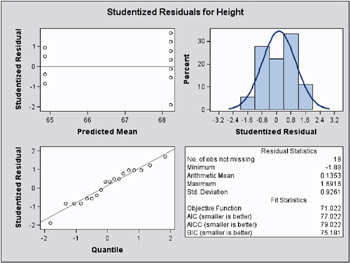
Figure 46.15: Marginal Studentized Residual Panel (Experimental)

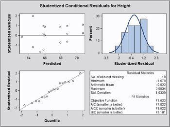
Figure 46.16: Conditional Studentized Residual Panel (Experimental)

A similar panel display for the scaled residuals is produced when you specify the experimental VCIRY option of the MODEL statement; see option VCIRY on page 2705 for more details.

The Residual Statistics in the lower right-hand corner inset provides descriptive statistics for the set of residuals that is displayed. Note that residuals in a mixed model do not necessarily sum to zero, even if the model contains an intercept.

Influence Plots

With the experimental graphics features the MIXED procedure can generate one or more panels of influence graphics. The type and number of panels produced depends on the modifiers of the INFLUENCE option. Plots related to covariance parameters are produced when diagnostics are computed by iterative methods (ITER=). The estimates of the fixed effects ”and covariance parameters when updates are iterative ” are plotted when the ESTIMATES modifier is specified.

The two types of panel graphs produced by the INFLUENCE option are shown in Figure 46.17 and Figure 46.18. The diagnostics panel shows an overall influence statistic (likelihood distance) and diagnostics for the fixed effects (CookD and COVRATIO). The statistics produced depend on suboptions of the INFLUENCE option (see Example 46.8 for the statements and options that produced Figure 46.17). Reference lines are drawn at zero for PRESS residuals and COVTRACE, and at one for COVRATIO. A reference line for likelihood distances is drawn at the 75th percentile of a chi-square distribution with m degrees of freedom if the largest displacement value in the Influence table is close to or larger than that percentile. The number m equals the number of parameters being updated.

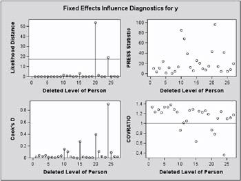
Figure 46.17: Influence Diagnostics (Experimental)

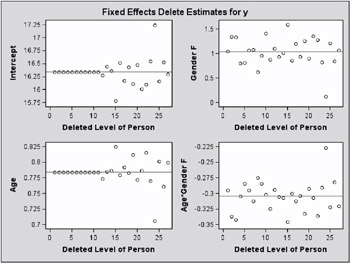
Figure 46.18: Delete Estimates (Experimental)

The second type of influence panel plot is obtained when you specify the ESTIMATES suboption (Figure 46.18). It shows the delete-estimates for each updated model parameter. Reference lines are drawn at the full data estimates. For noniterative influence analyses with profiled residual variance, the delete-case root mean square error is also plotted.

For the SAS statements that produce influence plots and for variations of these graphs see Example 46.7 and Example 46.8.

Box Plots

You can specify the BOXPLOT option in the PROC MIXED statement.

• BOXPLOT < ( suboptions ) >

  • requests box plots of observed and residual values Y ˆ’ X for effects that consist of single CLASS variables. This includes SUBJECT= and GROUP= effects.

  • For models with a RANDOM statement you also obtain box plots of the conditional residuals Y ˆ’ X ˆ’ Z . The box plots are constructed from studentized residuals when the RESIDUAL option of the MODEL statement is specified.

  • The following suboptions modify the appearance of the plots:

  • DATALABEL NODATALABEL

    • determines whether to place observation labels next to far outliers. Far outliers are labeled by default.

  • FILL NOFILL

    • determines whether the boxes are filled. The default is FILL.

  • NPANEL= n

    • limits the number of boxes per plot. The default is to place box plots for all levels of a factor in a common panel.

  • See Example 46.8 for an application.

ODS Graph Names

The MIXED procedure assigns a name to each graph it creates using ODS. You can use these names to reference the graphs when using ODS. The names are listed in Table 46.11.

To request these graphs, you must specify the ODS GRAPHICS statement in addition to the options indicated in Table 46.11. For more information on the ODS GRAPHICS statement, see Chapter 15, Statistical Graphics Using ODS.

Residuals and Influence Diagnostics (Experimental)

Residual Diagnostics

Consider a residual vector of the form = PY , where P is a projection matrix, possibly an oblique projector. A typical element with variance v _i and estimated variance _i is said to be standardized as

and studentized as

External studentization uses an estimate of var[ ] which does not involve the i th observation. Externally studentized residuals are often preferred over studentized residuals because they have well-known distributional properties in standard linear models for independent data.

Residuals that are scaled by the estimated variance of the response, i.e., , are referred to as Pearson-type residuals.

Marginal and Conditional Residuals

The marginal and conditional means in the linear mixed model are E[ Y ]= X ² and E[ Y ³ ]= X ² + Z ³ , respectively. Accordingly, the vector r _m of marginal residuals is defined as

and the vector r _c of conditional residuals is

Following Gregoire, Schabenberger, and Barrett (1995), let Q = X(X ² ^{ˆ’ 1} X) ^ˆ’ X ² and K = I ˆ’ Z Z ² ^{ˆ’ 1} . Then

For an individual observation the raw, studentized, and Pearson residuals computed by the RESIDUAL option of the MODEL statement are given in the following table.

Type of Residual	Marginal	Conditional
Raw
Studentized
Pearson

When the OUTPM= option of the MODEL statement is specified in addition to the RESIDUAL option, r _mi , , and are added to the data set as variables Resid , StudentResid , and PearsonResid , respectively. When the OUTP= option is specified, r _ci , , and are added to the data set.

Scaled Residuals

For correlated data, a set of scaled quantities can be defined through the Cholesky decomposition of the variance-covariance matrix. Since fitted residuals in linear models are rank- deficient , it is customary to draw on the variance-covariance matrix of the data. If var[ Y ] = V and C ² C = V , then C ² ^{ˆ’ 1} Y has uniform dispersion and its elements are uncorrelated.

Scaled residuals in a mixed model are meaningful for quantities based on the marginal distribution of the data. Let denote the Cholesky root of , so that ² = , and define

By analogy with other scalings, the inverse Cholesky decomposition can also be applied to the residual vector, ² ^{ˆ’ 1} r _m, although V is not the variance-covariance matrix of r _m .

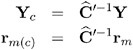
To diagnose whether the covariance structure of the model has been specified correctly can be difficult based on Y _c , since the inverse Cholesky transformation affects the expected value of Y _c . You can draw on r _m ( c ) as a vector of (approximately) uncorrelated data with constant mean.

When the OUTPM= option of the MODEL statement is specified in addition to the VCIRY option, Y _c is added as variable ScaledDep and r _{m ( c )} is added as ScaledResid to the data set.

Influence Diagnostics

The Basic Idea and Statistics

The general idea of quantifying the influence of one or more observations relies on computing parameter estimates based on all data points, removing the cases in question from the data, refitting the model, and computing statistics based on the change between full-data and reduced-data estimation. Influence statistics can be coarsely grouped by the aspect of estimation which is their primary target:

• overall measures compare changes in objective functions: (restricted) likelihood distance (Cook and Weisberg 1982, Ch. 5.2)

• influence on parameter estimates: Cook s D (Cook 1977, 1979), MDFFITS (Belsley, Kuh, and Welsch 1980, p. 32)

• influence on precision of estimates: CovRatio and CovTrace

• influence on fitted and predicted values: PRESS residual, PRESS statistic (Allen 1974), DFFITS (Belsley, Kuh, and Welsch 1980, p. 15)

• outlier properties: Internally and externally studentized residuals, leverage

For linear models for uncorrelated data, it is not necessary to refit the model after removing a data point in order to measure the impact of an observation on the model. The change in fixed effect estimates, residuals, residual sums of squares, and the variance-covariance matrix of the fixed effects can be computed based on the fitto the full data alone. By contrast, in mixed models several important complications arise. Data points can impact not only the fixed effects but also the covariance parameter estimates on which the fixed effects estimates depend. Furthermore, closed-form expressions for computing the change in important model quantities may not be available.

This section provides background material for the various influence diagnostics available with the MIXED procedure. See the section Mixed Models Theory beginning on page 2731 for relevant expressions and definitions. The parameter vector denotes all unknown parameters in the R and G matrix.

The observations whose influence is being ascertained are represented by the set U and referred to simply as the observations in U . The estimate of a parameter vector, for example, ² , obtained from all observations except those in the set U is denoted _{( U )} . In case of a matrix A , the notation A _{( U )} represents the matrix with the rows in U removed; these rows are collected in A _U . If A is symmetric, then notation A _{( U )} implies removal of rows and columns. The vector Y _U comprises the responses of the data points being removed, and V _{( U )} is the variance-covariance matrix of the remaining observations. When k = 1, lowercase notation emphasizes that single points are removed, e.g., A _{( u )} .

Managing the Covariance Parameters

An important component of influence diagnostics in the mixed model is the estimated variance-covariance matrix V = ZGZ ² + R . To make the dependence on the vector of covariance parameters explicit, write it as V ( ). If one parameter, ƒ ² , is profiled or factored out of V , the remaining parameters are denoted as *. Notice that in a model where G is diagonal and R = ƒ ² I , the parameter vector * contains the ratios of each variance component and ƒ ² (see Wolfinger, Tobias, and Sall 1994). When ITER=0, two scenarios are distinguished:

1. If the residual variance is not profiled, either because the model does not contain a residual variance or because it is part of the Newton-Raphson iterations, then _{( U )} ‰ .

2. If the residual variance is profiled then ^* _{( U )} ‰ ^* and . Influence statistics such as Cook s D and internally studentized residuals are based on V ( ) whereas externally studentized residuals and the DFFITS statistic are based on . In a random components model with uncorrelated errors, for example, the computation of V ( _U ) involves scaling of and by the full data estimate ² and multiplying the result with the reduced-data estimate .

Certain statistics, such as MDFFITS, COVRATIO, and COVTRACE, require an estimate of the variance of the fixed effects that is based on the reduced number of observations. For example, V ( _U ) is evaluated at the reduced-data parameter estimates but computed for the entire data set. The matrix V _{( U )} ( _{( U )} ), on the other hand, has rows and columns corresponding to the points in U removed. The resulting matrix is evaluated at the delete-case estimates.

When influence analysis is iterative, the entire vector is updated, whether the residual variance is profiled or not. The matrices to be distinguished here are V ( ), V ( _{( U )} ), and V _{( U )} ( _{( U )} ), with unambiguous notation.

Predicted Values, PRESS Residual, and PRESS Statistic

An unconditional predicted value is , where the vector x _i is the i th row of X . The (raw) residual is given as and the PRESS residual is

The PRESS statistic is the sum of the squared PRESS residuals,

where the sum is over the observations in U .

If EFFECT=, SIZE=, or KEEP= are not specified, PROC MIXED computes the PRESS residual for each observation selected through SELECT= (or all observations if SELECT= is not given). If EFFECT=, SIZE =, or KEEP= are specified, the procedure computes PRESS .

Leverage

For the general mixed model, leverage can be defined through the projection matrix that results from a transformation of the model with the inverse of the Cholesky decomposition of V , or through an oblique projector. The MIXED procedure follows the latter path in the computation of influence diagnostics. The leverage value reported for the i th observation is the i th diagonal entry of the matrix

which is the weight of the observation in contributing to its own predicted value, H = d / d Y .

While H is idempotent, it is generally not symmetric and thus not a projection matrix in the narrow sense.

The properties of these leverages are generalizations of the properties in models with diagonal variance-covariance matrices. For example, = HY , and in a model with intercept and V = ƒ ² I , the leverage values

are and rank( X ). The lower bound for h _ii is achieved in an intercept-only model, the upper bound in a saturated model. The trace of H equals the rank of X .

If ½ _ij denotes the element in row i , column j of V ^{ˆ’ 1} , then for a model containing only an intercept the diagonal elements of H are

Because is a sum of elements in the i th row of the inverse variance-covariance matrix h _ii can be negative, even if the correlations among data points are nonnegative. In case of a saturated model with X = I , h _ii =1 . 0.

Internally and Externally Studentized Residuals

See the section Residual Diagnostics on page 2763 for the distinction between standardization, studentization, and scaling of residuals. Internally studentized marginal and conditional residuals are computed with the RESIDUAL option of the MIXED procedure (p. 2763). The INFLUENCE option computes internally and externally studentized marginal residuals.

The computation of internally studentized residuals relies on the diagonal entries of V( ) ˆ’ Q( ) where Q( ) = X(X ² V( ) ^{ˆ’ 1} X) ^ˆ’ X ² . Externally studentized residuals require iterative influence analysis or a profiled residual variance. In the former case the studentization is based on V ( _U ); in the latter case it is based on .

Cook s D

Cook s D statistic is an invariant norm that measures the influence of observations in U on a vector of parameter estimates (Cook 1977). In case of the fixed effects coefficients, let

Then the MIXED procedure computes

where is the matrix that results from sweeping (X ² V( ) ^{ˆ’ 1} X) ^ˆ’ .

If V is known, Cook s D can be calibrated according to a chi-square distribution with degrees of freedom equal to the rank of X (Christensen, Pearson, and Johnson 1992). For estimated V the calibration can be carried out according to an F (rank( X ), n ˆ’ rank( X )) distribution. To interpret D on a familiar scale, Cook (1979) and Cook and Weisberg (1982, p. 116) refer to the 50th percentile of the reference distribution. If D is equal to that percentile, then removing the points in U moves the fixed effects coefficient vector from the center of the confidence region to the 50% confidence ellipsoid (Myers 1990, p. 262).

In the case of iterative influence analysis, the MIXED procedure also computes a D -type statistic for the covariance parameters. If “ is the asymptotic variance-covariance matrix of , then MIXED computes

DFFITS and MDFFITS

A DFFIT measures the change in predicted values due to removal of data points. If this change is standardized by the externally estimated standard error of the predicted value in the full data, the DFFITS statistic of Belsley, Kuh, and Welsch (1980, p. 15) results:

The MIXED procedure computes DFFITS when the EFFECT= or SIZE= modifiers of the INFLUENCE option are not in effect. In general, an external estimate of the estimated standard error is used. When ITER > 0, the estimate is

When ITER=0 and ƒ ² is profiled, then

When the EFFECT=, SIZE=, or KEEP= modifiers are specified, the MIXED procedure computes a multivariate version suitable for the deletion of multiple data points. The statistic, termed MDFFITS after the MDFFIT statistic of Belsley, Kuh, and Welsch (1980, p. 32), is closely related to Cook s D . Consider the case V = ƒ ² V ( *) so that

and let be an estimate of var[ _{( U )} ] that does not use the observations in U . The MDFFITS statistic is then computed as

If ITER=0 and ƒ ² is profiled, then is obtained by sweeping

The underlying idea is that if * were known, then

would be [ ] / ƒ ² in a generalized least squares regression with all but the data in U .

In the case of iterative influence analysis, is evaluated at _{( U )} . Furthermore, a MDFFITS-type statistic is then computed for the covariance parameters:

Covariance Ratio and Trace

These statistics depend on the availability of an external estimate of V , or at least of ƒ ² . Whereas Cook s D and MDFFITS measure the impact of data points on a vector of parameter estimates, the covariance-based statistics measure impact on their precision. Following Christensen, Pearson, and Johnson (1992), the MIXED procedure computes

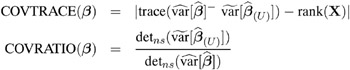
where det _ns ( M ) denotes the determinant of the nonsingular part of matrix M .

In the case of iterative influence analysis these statistics are also computed for the covariance parameter estimates. If q denotes the rank of var[ ], then

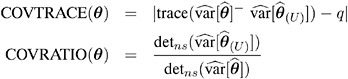
Likelihood Distances

The log-likelihood function l and restricted log-likelihood function l _R of the linear mixed model are given in the section Estimating G and R in the Mixed Model beginning on page 2737. Denote as ˆ the collection of all parameters, i.e., the fixed effects ² and the covariance parameters . Twice the difference between the (restricted) log-likelihood evaluated at the full-data estimates and at the reduced-data estimates _{( U )} is known as the (restricted) likelihood distance:

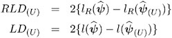
Cook and Weisberg (1982, Ch. 5.2) refer to these differences as likelihood distances , Beckman, Nachtsheim, and Cook (1987) term the measures likelihood displacements . If the number of elements in ˆ that are subject to updating following point removal is q , then likelihood displacements can be compared against cutoffs from a chi-square distribution with q degrees of freedom. Notice that this reference distribution does not depend on the number of observations removed from the analysis, but rather on the number of model parameters that are updated. The likelihood displacement gives twice the amount by which the log-likelihood of the full data changes if one were to utilize an estimate based on fewer data points. It is thus a global, summary measure of the influence of the observations in U jointly on all parameters.

Unless METHOD=ML, the MIXED procedure computes the likelihood displacement based on the residual (=restricted) log likelihood, even if METHOD=MIVQUE0 or METHOD=TYPE1, TYPE2, or TYPE3.

Noniterative Update Formulas

Update formulas that do not require refitting of the model are available for the cases where V = ƒ ² I , V is known, or V * is known. When ITER=0 and these update formulas can be invoked, the MIXED procedure uses the computational devices that are outlined in the following paragraphs. It is then assumed that the variance-covariance matrix of the fixed effects has the form ( X ² V ^{ˆ’ 1} X ) ˆ’ . When DDFM=KENWARDROGER, this is not the case; the estimated variance-covariance matrix is then inflated to better represent the uncertainty in the estimated covariance parameters. Influence statistics when DDFM=KENWARDROGER should iteratively update the covariance parameters (ITER > 0). The dependence of V on is suppressed in the sequel for brevity.

Updating the Fixed Effects

Denote by U the ( n — k ) matrix that is assembled from k columns of the identity matrix. Each column of U corresponds to the removal of one data point. The point being targeted by the i th column of U corresponds to the row in which a 1 appears. Furthermore, define

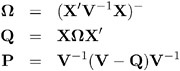
The change in the fixed effects estimates following removal of the observations in U is

Using results in Cook and Weisberg (1982, A2) you can further compute

if X is ( n — p ) of rank m < p , then is deficient in rank and the MIXED procedure computes needed quantities in iconid=pb50 by sweeping (Goodnight 1979). If the rank of the ( k — k ) matrix U ² PU is less than k , the removal of the observations introduces a new singularity, whether X is of full rank or not. The solution vectors and _{( U )} then do not have the same expected values and should not be compared. When the MIXED procedure encounters this situation, influence diagnostics that depend on the choice of generalized inverse are not computed. The procedure also monitors the singularity criteria when sweeping the rows of ( X ² V ^{ˆ’ 1} X ) ^ˆ’ and of ( ) ˆ’ . If a new singularity is encountered or a former singularity disappears, no influence statistics are computed.

Residual Variance

When ƒ ² is profiled out of the marginal variance-covariance matrix, a closed-form estimate of ƒ ² that is based on only the remaining observations can be computed provided V * = V ( ^* ) is known. Hurtado (1993, Thm. 5.2) shows that

and _U = U ² V* ^{ˆ’ 1} (y ˆ’ X ). In the case of maximum likelihood estimation q = 0 and for REML estimation q = rank( X ). The constant r equals the rank of ( U ² PU ) for REML estimation and the number of effective observations that are removed if METHOD=ML.

Likelihood Distances

For noniterative methods the following computational devices are used to compute (restricted) likelihood distances provided that the residual variance ƒ ² is profiled.

The log-likelihood function l ( ) evaluated at the full-data and reduced-data estimates can be written as

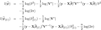
Notice that l ( _{( U )} ) evaluates the log-likelihood for n data points at the reduced-data estimates. It is not the log-likelihood obtained by fitting the model to the reduced data. The likelihood distance is then

Expressions for RLD _{( U )} in noniterative influence analysis are derived along the same lines.

Computational Issues

Computational Method

In addition to numerous matrix-multiplication routines, PROC MIXED frequently uses the sweep operator (Goodnight 1979) and the Cholesky root (Golub and Van Loan 1989). The routines perform a modified W transformation (Goodnight and Hemmerle 1979) for G -side likelihood calculations and a direct method for R -side likelihood calculations. For the Type III F -tests, PROC MIXED uses the algorithm described in Chapter 32, The GLM Procedure.

PROC MIXED uses a ridge-stabilized Newton-Raphson algorithm to optimize either a full (ML) or residual (REML) likelihood function. The Newton-Raphson algorithm is preferred to the EM algorithm (Lindstrom and Bates 1988). PROC MIXED profiles the likelihood with respect to the fixed effects and also with respect to the residual variance whenever it appears reasonable to do so. The residual profiling can be avoided by using the NOPROFILE option of the PROC MIXED statement. PROC MIXED uses the MIVQUE0 method (Rao 1972; Giesbrecht 1989) to compute initial values.

The likelihoods that PROC MIXED optimizes are usually well-defined continuous functions with a single optimum. The Newton-Raphson algorithm typically performs well and finds the optimum in a few iterations. It is a quadratically converging algorithm, meaning that the error of the approximation near the optimum is squared at each iteration. The quadratic convergence property is evident when the convergence criterion drops to zero by factors of 10 or more.

Table 46.12: Notation for Order Calculations

Symbol	Number
p	columns of X
g	columns of Z
N	observations
q	covariance parameters
t	maximum observations per subject
S	subjects

Using the notation from Table 46.12, the following are estimates of the computational speed of the algorithms used in PROC MIXED. For likelihood calculations, the crossproducts matrix construction is of order N ( p + g ) ² and the sweep operations are of order ( p + g ) ³ .Thefirst derivative calculations for parameters in G are of order qg ³ for ML and q ( g ³ + pg ² + p ² g ) for REML. If you specify a subject effect in the RANDOM statement and if you are not using the REPEATED statement, then replace g by g/S and q by qS in these calculations. The first derivative calculations for parameters in R are of order qS ( t ³ + gt ² + g ² t ) for ML and qS ( t ³ +( p + g ) t ² +( p ² + g ² ) t ) for REML. For the second derivatives, replace q by q ( q +1) / 2 in the first derivative expressions. When you specify both G -and R -side parameters (that is, when you use both the RANDOM and REPEATED statements), then additional calculations are required of an order equal to the sum of the orders for G and R . Considerable execution times may result in this case.

For further details about the computational techniques used in PROC MIXED, refer to Wolfinger, Tobias, and Sall (1994).

Parameter Constraints

By default, some covariance parameters are assumed to satisfy certain boundary constraints during the Newton-Raphson algorithm. For example, variance components are constrained to be nonnegative and autoregressive parameters are constrained to be between ˆ’ 1 and 1. You can remove these constraints with the NOBOUND option in the PARMS statement, but this may lead to estimates that produce an infinite likelihood. You can also introduce or change boundary constraints with the LOWERB= and UPPERB= options in the PARMS statement.

During the Newton-Raphson algorithm, a parameter may be set equal to one of its boundary constraints for a few iterations and then it may move away from the boundary. You see a missing value in the Criterion column of the Iteration History table whenever a boundary constraint is dropped.

For some data sets the final estimate of a parameter may equal one of its boundary constraints. This is usually not a cause for concern, but it may lead you to consider a different model. For instance, a variance component estimate can equal zero; in this case, you may want to drop the corresponding random effect from the model. However, be aware that changing the model in this fashion can impact degrees of freedom calculations.

Convergence Problems

For some data sets, the Newton-Raphson algorithm can fail to converge. Non-convergence can result from a number of causes, including flat or ridged likelihood surfaces and ill-conditioned data.

It is also possible for PROC MIXED to converge to a point that is not the global optimum of the likelihood, although this usually occurs only with the spatial covariance structures.

If you experience convergence problems, the following points may be helpful:

• One useful tool is the PARMS statement, which lets you input initial values for the covariance parameters and performs a grid search over the likelihood surface.

• Sometimes the Newton-Raphson algorithm does not perform well when two of the covariance parameters are on a different scale; that is, they are several orders of magnitude apart. This is because the Hessian matrix is processed jointly for the two parameters, and elements of it corresponding to one of the parameters can become close to internal tolerances in PROC MIXED. In this case, you can improve stability by rescaling the effects in the model so that the covariance parameters are on the same scale.

• Data that is extremely large or extremely small can adversely affect results because of the internal tolerances in PROC MIXED. Rescaling it can improve stability.

• For stubborn problems, you may want to specify ODS OUTPUT COVPARMS= data-set-name to output the CovParms table as a precautionary measure. That way, if the problem does not converge, you can read the final parameter values back into a new run with the PARMSDATA= option in the PARMS statement.

• Fisher scoring can be more robust than Newton-Raphson to poor MIVQUE(0) starting values. Specifying a SCORING= value of 5 or so may help to recover from poor starting values.

• Tuning the singularity options SINGULAR=, SINGCHOL=, and SINGRES= in the MODEL statement may improve the stability of the optimization process.

• Tuning the MAXITER= and MAXFUNC= options in the PROC MIXED statement can save resources. Also, the ITDETAILS option displays the values of all of the parameters at each iteration.

• Using the NOPROFILE and NOBOUND options in the PROC MIXED statement may help convergence, although they can produce unusual results.

• Although the CONVH convergence criterion usually gives the best results, you may want to try CONVF or CONVG, possibly along with the ABSOLUTE option.

• If the convergence criterion bottoms out at a relatively small value such as 1E ˆ’ 7 but never gets less than 1E ˆ’ 8, you may want to specify CONVH=1E ˆ’ 6 in the PROC MIXED statement to get results; however, interpret the results with caution.

• An infinite likelihood during the iteration process means that the Newton-Raphson algorithm has stepped into a region where either the R or V matrix is nonpositive definite. This is usually no cause for concern as long as iterations continue. If PROC MIXED stops because of an infinite likelihood, recheck your model to make sure that no observations from the same subject are producing identical rows in R or V and that you have enough data to estimate the particular covariance structure you have selected. Any time that the final estimated likelihood is infinite, subsequent results should be interpreted with caution.

• A nonpositive definite Hessian matrix can indicate a surface saddlepoint or linear dependencies among the parameters.

• A warning message about the singularities of X changing indicates that there is some linear dependency in the estimate of X ² ^{ˆ’ 1} X that is not found in X ² X . This can adversely affect the likelihood calculations and optimization process. If you encounter this problem, make sure that your model specification is reasonable and that you have enough data to estimate the particular covariance structure you have selected. Rearranging effects in the MODEL statement so that the most significant ones are first can help because PROC MIXED sweeps the estimate of X ² V ^{ˆ’ 1} X in the order of the MODEL effects and the sweep is more stable if larger pivots are dealt with first. If this does not help, specifying starting values with the PARMS statement can place the optimization on a different and possibly more stable path.

• Lack of convergence may indicate model misspecification or a violation of the normality assumption.

Memory

Let p be the number of columns in X , and let g be the number of columns in Z . For large models, most of the memory resources are required for holding symmetric matrices of order p , g , and p + g . The approximate memory requirement in bytes is

If you have a large model that exceeds the memory capacity of your computer, see the suggestions listed under Computing Time.

Computing Time

PROC MIXED is computationally intensive , and execution times can be long. In addition to the CPU time used in collecting sums and cross products and in solving the mixed model equations (as in PROC GLM), considerable CPU time is often required to compute the likelihood function and its derivatives. These latter computations are performed for every Newton-Raphson iteration.

If you have a model that takes too long to run, the following suggestions may be helpful:

• Examine the Model Information table to find out the number of columns in the X and Z matrices. A large number of columns in either matrix can greatly increase computing time. You may want to eliminate some higher order effects if they are too large.

• If you have a Z matrix with a lot of columns, use the DDFM=BW optioninthe MODEL statement to eliminate the time required for the containment method.

• If possible, factor out a common effect from the effects in the RANDOM statement and make it the SUBJECT= effect. This creates a block-diagonal G matrix and can often speed calculations.

• If possible, use the same or nested SUBJECT= effects in all RANDOM and REPEATED statements.

• If your data set is very large, you may want to analyze it in pieces. The BY statement can help implement this strategy.

• In general, specify random effects with a lot of levels in the REPEATED statement and those with a few levels in the RANDOM statement.

• The METHOD=MIVQUE0 option runs faster than either the METHOD=REML or METHOD=ML option because it is noniterative.

• You can specify known values for the covariance parameters using the HOLD= or NOITER option in the PARMS statement or the GDATA= option in the RANDOM statement. This eliminates the need for iteration.

• The LOGNOTE option in the PROC MIXED statement writes periodic messages to the SAS log concerning the status of the calculations. It can help you diagnose where the slow down is occurring.