Examples
The following are basic examples of the use of PROC MIXED. More examples and details can be found in Littell et al. (1996), Wolfinger (1997), Verbeke and Molenberghs (1997, 2000), Murray (1998), Singer (1998), Sullivan, Dukes, and Losina (1999), and Brown and Prescott (1999).
Example 46.1. Split-Plot Design
PROC MIXED can fit a variety of mixed models. One of the most common mixed models is the split-plot design. The split-plot design involves two experimental factors, A and B .Levelsof A are randomly assigned to whole plots (main plots), and levels of B are randomly assigned to split plots (subplots) within each whole plot. The design provides more precise information about B than about A , and it often arises when A can be applied only to large experimental units. An example is where A represents irrigation levels for large plots of land and B represents different crop varieties planted in each large plot.
Consider the following data from Stroup (1989a), which arise from a balanced split-plot design with the whole plots arranged in a randomized complete-block design. The variable A is the whole-plot factor, and the variable B is the subplot factor. A traditional analysis of these data involves the construction of the whole-plot error ( A * Block )totest A and the pooled residual error ( B * Block and A * B * Block )totest B and A * B . To carry out this analysis with PROC GLM, you must use a TEST statement to obtain the correct F -test for A .
Performing a mixed model analysis with PROC MIXED eliminates the need for the error term construction. PROC MIXED estimates variance components for Block , A * Block , and the residual, and it automatically incorporates the correct error terms into test statistics.
data sp; input Block A B Y @@; datalines; 1 1 1 56 1 1 2 41 1 2 1 50 1 2 2 36 1 3 1 39 1 3 2 35 2 1 1 30 2 1 2 25 2 2 1 36 2 2 2 28 2 3 1 33 2 3 2 30 3 1 1 32 3 1 2 24 3 2 1 31 3 2 2 27 3 3 1 15 3 3 2 19 4 1 1 30 4 1 2 25 4 2 1 35 4 2 2 30 4 3 1 17 4 3 2 18 ;
proc mixed; class A B Block; model Y = A B A*B; random Block A*Block; run;
The variables A , B , and Block are listed as classification variables in the CLASS statement. The columns of model matrix X consist of indicator variables corresponding to the levels of the fixed effects A , B , and A * B listed on the right-hand side in the MODEL statement. The dependent variable Y is listed on the left-hand side in the MODEL statement.
The columns of the model matrix Z consist of indicator variables corresponding to the levels of the random effects Block and A * Block .The G matrix is diagonal and contains the variance components of Block and A * Block .The R matrix is also diagonal and contains the residual variance.
The SAS code produces Output 46.1.1.
| |
The Mixed Procedure Model Information Data Set WORK.SP Dependent Variable Y Covariance Structure Variance Components Estimation Method REML Residual Variance Method Profile Fixed Effects SE Method Model-Based Degrees of Freedom Method Containment
| |
The Model Information table lists basic information about the split-plot model. REML is used to estimate the variance components, and the residual variances are profiled out of the optimization.
The Mixed Procedure Class Level Information Class Levels Values A 3 1 2 3 B 2 1 2 Block 4 1 2 3 4
The Class Level Information table lists the levels of all variables specified in the CLASS statement. You can check this table to make sure that the data are correct.
The Mixed Procedure Dimensions Covariance Parameters 3 Columns in X 12 Columns in Z 16 Subjects 1 Max Obs Per Subject 24
The Dimensions table lists the magnitudes of various vectors and matrices. The X matrix is seen to be 24 — 12, and the Z matrix is 24 — 16.
The Mixed Procedure Number of Observations Number of Observations Read 24 Number of Observations Used 24 Number of Observations Not Used 0
The Number of Observations table shows that all observations read from the data set are used in the analysis.
The Mixed Procedure Iteration History Iteration Evaluations -2 Res Log Like Criterion 0 1 139.81461222 1 1 119.76184570 0.00000000 Convergence criteria met.
PROC MIXED estimates the variance components for Block , A * Block , and the residual by REML. The REML estimates are the values that maximize the likelihood of a set of linearly independent error contrasts, and they provide a correction for the downward bias found in the usual maximum likelihood estimates. The objective function is ˆ’ 2 times the logarithm of the restricted likelihood, and PROC MIXED minimizes this objective function to obtain the estimates.
The minimization method is the Newton-Raphson algorithm, which uses the first and second derivatives of the objective function to iteratively find its minimum. The Iteration History table records the steps of that optimization process. For this example, only one iteration is required to obtain the estimates. The Evaluations column reveals that the restricted likelihood is evaluated once for each of the iterations. A criterion of 0 indicates that the Newton-Raphson algorithm has converged .
The Mixed Procedure Covariance Parameter Estimates Cov Parm Estimate Block 62.3958 A*Block 15.3819 Residual 9.3611
The REML estimates for the variance components of Block , A * Block , and the residual are 62.40, 15.38, and 9.36, respectively, as listed in the Estimate column of the Covariance Parameter Estimates table.
The Mixed Procedure Fit Statistics -2 Res Log Likelihood 119.8 AIC (smaller is better) 125.8 AICC (smaller is better) 127.5 BIC (smaller is better) 123.9
The Fitting Information table lists several pieces of information about the fitted mixed model, including the residual log likelihood. Akaike s and Schwarz s criteria can be used to compare different models; the ones with smaller values are preferred.
The Mixed Procedure Type 3 Tests of Fixed Effects Num Den Effect DF DF F Value Pr > F A 2 6 4.07 0.0764 B 1 9 19.39 0.0017 A*B 2 9 4.02 0.0566
Finally, the fixed effects are tested using Type III estimable functions. The tests match the one obtained from the following PROC GLM code:
proc glm data=sp; class A B Block; model Y = A B A*B Block A*Block; test h=A e=A*Block; run;
You can continue this analysis by producing solutions for the fixed and random effects and then testing various linear combinations of them by using the CONTRAST and ESTIMATE statements. If you use the same CONTRAST and ESTIMATE statements with PROC GLM, the test statistics correspond to the fixed-effects-only model. The test statistics from PROC MIXED incorporate the random effects.
The various inference space contrasts given by Stroup (1989a) can be implemented via the ESTIMATE statement. Consider the following examples:
estimate a1 mean narrow intercept 1 A 1 B .5 .5 A*B .5 .5 Block .25 .25 .25 .25 A*Block .25 .25 .25 .25 0 0 0 0 0 0 0 0; estimate a1 mean intermed intercept 1 A 1 B .5 .5 A*B .5 .5 Block .25 .25 .25 .25; estimate a1 mean broad intercept 1 a 1 b .5 .5 A*B .5 .5;
These statements result in Output 46.1.2.
| |
The Mixed Procedure Estimates Standard Label Estimate Error DF t Value Pr > t a1 mean narrow 32.8750 1.0817 9 30.39 <.0001 a1 mean intermed 32.8750 2.2396 9 14.68 <.0001 a1 mean broad 32.8750 4.5403 9 7.24 <.0001
| |
Note that all the estimates are equal, but their standard errors increase with the size of the inference space. The narrow inference space consists of the observed levels of Block and A * Block , and the t -statistic value of 30.39 applies only to these levels. This is the same t -statistic computed by PROC GLM, because it computes standard errors from the narrow inference space. The intermediate inference space consists of the observed levels of Block and the entire population of levels from which A * Block are sampled. The t -statistic value of 14.68 applies to this intermediate space. The broad inference space consists of arbitrary random levels of both Block and A * Block , and the t -statistic value of 7.24 is appropriate. Note that the larger the inference space, the weaker the conclusion. However, the broad inference space is usually the one of interest, and even in this space conclusive results are common. The highly significant p -value for a1 mean broad is an example. You can also obtain the a1 mean broad result by specifying A in an LSMEANS statement. For more discussion of the inference space concept, refer to McLean, Sanders, and Stroup (1991).
The following statements illustrate another feature of the RANDOM statement. Recall that the basic code for a split-plot design with whole plots arranged in randomized blocks is as follows .
proc mixed; class A B Block; model Y = A B A*B; random Block A*Block; run;
An equivalent way of specifying this model is
proc mixed data=sp; class A B Block; model Y = A B A*B; random intercept A / subject=Block; run;
In general, if all of the effects in the RANDOM statement can be nested within one effect, you can specify that one effect using the SUBJECT= option. The subject effect is, in a sense, factored out of the random effects. The specification using the SUBJECT= effect can result in quicker execution times for large problems because PROC MIXED is able to perform the likelihood calculations separately for each subject.
Example 46.2. Repeated Measures
The following data are from Pothoff and Roy (1964) and consist of growth measurements for 11 girls and 16 boys at ages 8, 10, 12, and 14. Some of the observations are suspect (for example, the third observation for person 20); however, all of the data are used here for comparison purposes.
The analysis strategy employs a linear growth curve model for the boys and girls as well as a variance-covariance model that incorporates correlations for all of the observations arising from the same person. The data are assumed to be Gaussian, and their likelihood is maximized to estimate the model parameters. Refer to Jennrich and Schluchter (1986), Louis (1988), Crowder and Hand (1990), Diggle, Liang, and Zeger (1994), and Everitt (1995) for overviews of this approach to repeated measures. Jennrich and Schluchter present results for the Pothoff and Roy data from various covariance structures. The PROC MIXED code to fit an unstructured variance matrix (their Model 2) is as follows:
data pr; input Person Gender $ y1 y2 y3 y4; y=y1; Age=8; output; y=y2; Age=10; output; y=y3; Age=12; output; y=y4; Age=14; output; drop y1-y4; datalines; 1 F 21.0 20.0 21.5 23.0 2 F 21.0 21.5 24.0 25.5 3 F 20.5 24.0 24.5 26.0 4 F 23.5 24.5 25.0 26.5 5 F 21.5 23.0 22.5 23.5 6 F 20.0 21.0 21.0 22.5 7 F 21.5 22.5 23.0 25.0 8 F 23.0 23.0 23.5 24.0 9 F 20.0 21.0 22.0 21.5 10 F 16.5 19.0 19.0 19.5 11 F 24.5 25.0 28.0 28.0 12 M 26.0 25.0 29.0 31.0 13 M 21.5 22.5 23.0 26.5 14 M 23.0 22.5 24.0 27.5 15 M 25.5 27.5 26.5 27.0 16 M 20.0 23.5 22.5 26.0 17 M 24.5 25.5 27.0 28.5 18 M 22.0 22.0 24.5 26.5 19 M 24.0 21.5 24.5 25.5 20 M 23.0 20.5 31.0 26.0 21 M 27.5 28.0 31.0 31.5 22 M 23.0 23.0 23.5 25.0 23 M 21.5 23.5 24.0 28.0 24 M 17.0 24.5 26.0 29.5 25 M 22.5 25.5 25.5 26.0 26 M 23.0 24.5 26.0 30.0 27 M 22.0 21.5 23.5 25.0 ; proc mixed data=pr method=ml covtest; class Person Gender; model y = Gender Age Gender*Age / s; repeated / type=un subject=Person r; run;
To follow Jennrich and Schluchter, this example uses maximum likelihood (METHOD=ML) instead of the default REML to estimate the unknown covariance parameters. The COVTEST option requests asymptotic tests of all of the covariance parameters.
The MODEL statement first lists the dependent variable Y . The fixed effects are then listed after the equals sign. The variable Gender requests a different intercept for the girls and boys, Age models an overall linear growth trend, and Gender * Age makes the slopes different over time. It is actually not necessary to specify Age separately, but doing so enables PROC MIXED to carry out a test for heterogeneous slopes. The S option requests the display of the fixed-effects solution vector.
The REPEATED statement contains no effects, taking advantage of the default assumption that the observations are ordered similarly for each subject. The TYPE=UN option requests an unstructured block for each SUBJECT= Person . The R matrix is, therefore, block diagonal with 27 blocks, each block consisting of identical 4 — 4 unstructured matrices. The 10 parameters of these unstructured blocks make up the covariance parameters estimated by maximum likelihood. The R option requests that the first block of R be displayed.
The results from this analysis are shown in Output 46.2.1.
| |
The Mixed Procedure Model Information Data Set WORK.PR Dependent Variable y Covariance Structure Unstructured Subject Effect Person Estimation Method ML Residual Variance Method None Fixed Effects SE Method Model-Based Degrees of Freedom Method Between-Within
| |
The covariance structure is listed as Unstructured here, and no residual variance is used with this structure. The default degrees-of-freedom method here is Between-Within.
The Mixed Procedure Class Level Information Class Levels Values Person 27 1 2 3 4 5 6 7 8 9 10 11 12 13 14 15 16 17 18 19 20 21 22 23 24 25 26 27 Gender 2 F M
Note that Person has 27 levels and Gender has 2.
The Mixed Procedure Dimensions Covariance Parameters 10 Columns in X 6 Columns in Z 0 Subjects 27 Max Obs Per Subject 4
The 10 covariance parameters result from the 4 — 4 unstructured blocks of R . There is no Z matrix for this model, and each of the 27 subjects has a maximum of 4 observations.
The Mixed Procedure Number of Observations Number of Observations Read 108 Number of Observations Used 108 Number of Observations Not Used 0
The Mixed Procedure Iteration History Iteration Evaluations -2 Log Like Criterion 0 1 478.24175986 1 2 419.47721707 0.00000152 2 1 419.47704812 0.00000000 Convergence criteria met.
Three Newton-Raphson iterations are required to find the maximum likelihood estimates. The default relative Hessian criterion has a final value less than 1E ˆ’ 8, indicating the convergence of the Newton-Raphson algorithm and the attainment of an optimum.
The Mixed Procedure Estimated R Matrix for Person 1 Row Col1 Col2 Col3 Col4 1 5.1192 2.4409 3.6105 2.5222 2 2.4409 3.9279 2.7175 3.0624 3 3.6105 2.7175 5.9798 3.8235 4 2.5222 3.0624 3.8235 4.6180
The preceding 4 — 4 matrix is the estimated unstructured covariance matrix. It is the estimate of the first block of R , and the other 26 blocks all have the same estimate.
The Mixed Procedure Covariance Parameter Estimates Standard Z Cov Parm Subject Estimate Error Value Pr Z UN(1,1) Person 5.1192 1.4169 3.61 0.0002 UN(2,1) Person 2.4409 0.9835 2.48 0.0131 UN(2,2) Person 3.9279 1.0824 3.63 0.0001 UN(3,1) Person 3.6105 1.2767 2.83 0.0047 UN(3,2) Person 2.7175 1.0740 2.53 0.0114 UN(3,3) Person 5.9798 1.6279 3.67 0.0001 UN(4,1) Person 2.5222 1.0649 2.37 0.0179 UN(4,2) Person 3.0624 1.0135 3.02 0.0025 UN(4,3) Person 3.8235 1.2508 3.06 0.0022 UN(4,4) Person 4.6180 1.2573 3.67 0.0001
The preceding table lists the 10 estimated covariance parameters in order; note their correspondence to the first block of R displayed previously. The parameter estimates are labeled according to their location in the block in the Cov Parm column, and all of these estimates are associated with Person as the subject effect. The Std Error column lists approximate standard errors of the covariance parameters obtained from the inverse Hessian matrix. These standard errors lead to approximate Wald Z -statistics, which are compared with the standard normal distribution. The results of these tests indicate that all the parameters are significantly different from 0; however, the Wald test can be unreliable in small samples.
To carry out Wald tests of various linear combinations of these parameters, use the following procedure. First, run the code again, adding the ASYCOV option and an ODS statement:
ods output CovParms=cp AsyCov=asy; proc mixed data=pr method=ml covtest asycov; class Person Gender; model y = Gender Age Gender*Age / s; repeated / type=un subject=Person r; run;
This creates two data sets, cp and asy , which contain the covariance parameter estimates and their asymptotic variance covariance matrix, respectively. Then read these data sets into the SAS/IML matrix programming language as follows:
proc iml; use cp; read all var {Estimate} into est; use asy; read all var (CovP1:CovP10) into asy; You can then construct your desired linear combinations and corresponding quadratic forms with the asy matrix.
The Mixed Procedure Fit Statistics -2 Log Likelihood 419.5 AIC (smaller is better) 447.5 AICC (smaller is better) 452.0 BIC (smaller is better) 465.6 Null Model Likelihood Ratio Test DF Chi-Square Pr > ChiSq 9 58.76 <.0001
The null model likelihood ratio test (LRT) is highly significant for this model, indicating that the unstructured covariance matrix is preferred to the diagonal one of the ordinary least-squares null model. The degrees of freedom for this test is 9, which is the difference between 10 and the 1 parameter for the null model s diagonal matrix.
The Mixed Procedure Solution for Fixed Effects Standard Effect Gender Estimate Error DF t Value Pr > t Intercept 15.8423 0.9356 25 16.93 <.0001 Gender F 1.5831 1.4658 25 1.08 0.2904 Gender M 0 . . . . Age 0.8268 0.07911 25 10.45 <.0001 Age*Gender F -0.3504 0.1239 25 -2.83 0.0091 Age*Gender M 0 . . . .
The preceding table lists the solution vector for the fixed effects. The estimate of the boys intercept is 15 . 84, while that for the girls is 15 . 84+1 . 58 = 17 . 42. Similarly, the estimate for the boys slope is 0.827, while that for the girls is 0 . 827 ˆ’ . 350 = 0 . 477. Thus the girls starting point is larger than that for the boys, but their growth rate is about half that of the boys.
Note that two of the estimates equal 0; this is a result of the overparameterized model used by PROC MIXED. You can obtain a full-rank parameterization by using the following MODEL statement:
model y = Gender Gender*Age / noint s;
Here, the NOINT option causes the different intercepts to be fit directly as the two levels of Gender . However, this alternative specification results in different tests for these effects.
The Mixed Procedure Type 3 Tests of Fixed Effects Num Den Effect DF DF F Value Pr > F Gender 1 25 1.17 0.2904 Age 1 25 110.54 <.0001 Age*Gender 1 25 7.99 0.0091
The Type 3 Tests of Fixed Effects table displays Type III tests for all of the fixed effects. These tests are partial in the sense that they account for all of the other fixed effects in the model. In addition, you can use the HTYPE= option in the MODEL statement to obtain Type I (sequential) or Type II (also partial) tests of effects.
It is usually best to consider higher-order terms first, and in this case the Age * Gender test reveals a difference between the slopes that is statistically significant at the 1% level. Note that the p -value for this test (0 . 0091) is the same as the p -value in the Age*Gender F row in the Solution for Fixed Effects table and that the F -statistic (7 . 99) is the square of the t -statistic ( ˆ’ 2 . 83), ignoring rounding error. Similar connections are evident among the other rows in these two tables.
The Age test is one for an overall growth curve accounting for possible heterogeneous slopes, and it is highly significant. Finally, the Gender row tests the null hypothesis of a common intercept, and this hypothesis cannot be rejected from these data.
As an alternative to the F -tests shown here, you can carry out likelihood ratio tests of various hypotheses by fitting the reduced models, subtracting ˆ’ 2 log likelihoods, and comparing the resulting statistics with 2 distributions.
Since the different levels of the repeated effect represent different years , it is natural to try fitting a time series model to the data within each subject. To obtain time series structures in R , you can replace TYPE=UN with TYPE=AR(1) or TYPE=TOEP to obtain the first- or n th-order autoregressive covariance matrices, respectively. For example, the code to fit an AR(1) structure is
proc mixed data=pr method=ml; class Person Gender; model y = Gender Age Gender*Age / s; repeated / type=ar(1) sub=Person r; run;
To fit a random coefficients model, use the following code:
proc mixed data=pr method=ml; class Person Gender; model y = Gender Age Gender*Age / s; random intercept Age / type=un sub=Person g; run;
This specifies an unstructured covariance matrix for the random intercept and slope. In mixed model notation, G is block diagonal with identical 2 — 2 unstructured blocks for each person. By default, R becomes ƒ 2 I . See Example 46.5 for further information on this model.
Finally, you can fit a compound symmetry structure by using TYPE=CS.
proc mixed data=pr method=ml covtest; class Person Gender; model y = Gender Age Gender*Age / s; repeated / type=cs subject=Person r; run;
The results from this analysis are shown in Output 46.2.2.
| |
The Mixed Procedure Model Information Data Set WORK.PR Dependent Variable y Covariance Structure Compound Symmetry Subject Effect Person Estimation Method ML Residual Variance Method Profile Fixed Effects SE Method Model-Based Degrees of Freedom Method Between-Within
| |
The Model Information table is the same as before except for the change in Covariance Structure.
The Mixed Procedure Class Level Information Class Levels Values Person 27 1 2 3 4 5 6 7 8 9 10 11 12 13 14 15 16 17 18 19 20 21 22 23 24 25 26 27 Gender 2 F M Dimensions Covariance Parameters 2 Columns in X 6 Columns in Z 0 Subjects 27 Max Obs Per Subject 4 Number of Observations Number of Observations Read 108 Number of Observations Used 108 Number of Observations Not Used 0
The compound symmetry structure has two parameters.
The Mixed Procedure Iteration History Iteration Evaluations -2 Log Like Criterion 0 1 478.24175986 1 1 428.63905802 0.00000000 Convergence criteria met.
Since the data are balanced, only one step is required to find the estimates.
The Mixed Procedure Estimated R Matrix for Person 1 Row Col1 Col2 Col3 Col4 1 4.9052 3.0306 3.0306 3.0306 2 3.0306 4.9052 3.0306 3.0306 3 3.0306 3.0306 4.9052 3.0306 4 3.0306 3.0306 3.0306 4.9052
Note the compound symmetry structure here, which consists of a common covariance with a diagonal enhancement.
The Mixed Procedure Covariance Parameter Estimates Standard Z Cov Parm Subject Estimate Error Value Pr Z CS Person 3.0306 0.9552 3.17 0.0015 Residual 1.8746 0.2946 6.36 <.0001
The common covariance is estimated to be 3.0306, as listed in the CS row of the preceding table, and the residual variance is estimated to be 1.8746, as listed in the Residual row. You can use these two numbers to estimate the intraclass correlation coefficient (ICC) for this model. Here, the ICC estimate equals 3.0306/(3.0306 + 1.8746) = 0.6178. You can also obtain this number by adding the RCORR option to the REPEATED statement.
The Mixed Procedure Fit Statistics -2 Log Likelihood 428.6 AIC (smaller is better) 440.6 AICC (smaller is better) 441.5 BIC (smaller is better) 448.4 Null Model Likelihood Ratio Test DF Chi-Square Pr > ChiSq 1 49.60 <.0001
In this case, the null model LRT has only one degree of freedom, corresponding to the common covariance parameter. The test indicates that modeling this extra covariance is superior to fitting the simple null model.
The Mixed Procedure Solution for Fixed Effects Standard Effect Gender Estimate Error DF t Value Pr > t Intercept 16.3406 0.9631 25 16.97 <.0001 Gender F 1.0321 1.5089 25 0.68 0.5003 Gender M 0 . . . . Age 0.7844 0.07654 79 10.25 <.0001 Age*Gender F -0.3048 0.1199 79 -2.54 0.0130 Age*Gender M 0 . . . .
Note that the fixed effects estimates and their standard errors are not very different from those in the preceding unstructured example.
The Mixed Procedure Type 3 Tests of Fixed Effects Num Den Effect DF DF F Value Pr > F Gender 1 25 0.47 0.5003 Age 1 79 111.10 <.0001 Age*Gender 1 79 6.46 0.0130
The F -tests are also similar to those from the preceding unstructured example. Again, the slopes are significantly different but the intercepts are not.
You can fit the same compound symmetry model with the following specification using the RANDOM statement:
proc mixed data=pr method=ml; class Person Gender; model y = Gender Age Gender*Age / s; random Person; run;
Compound symmetry is the structure that Jennrich and Schluchter deemed best among the ones they fit. To carry the analysis one step further, you can use the GROUP = option to specify heterogeneity of this structure across girls and boys.
proc mixed data=pr method=ml; class Person Gender; model y = Gender Age Gender*Age / s; repeated / type=cs subject=Person group=Gender; run;
The results from this analysis are shown in Output 46.2.3.
| |
The Mixed Procedure Model Information Data Set WORK.PR Dependent Variable y Covariance Structure Compound Symmetry Subject Effect Person Group Effect Gender Estimation Method ML Residual Variance Method None Fixed Effects SE Method Model-Based Degrees of Freedom Method Between-Within
| |
Note that Gender is listed as a Group Effect.
The Mixed Procedure Class Level Information Class Levels Values Person 27 1 2 3 4 5 6 7 8 9 10 11 12 13 14 15 16 17 18 19 20 21 22 23 24 25 26 27 Gender 2 F M Dimensions Covariance Parameters 4 Columns in X 6 Columns in Z 0 Subjects 27 Max Obs Per Subject 4 Number of Observations Number of Observations Read 108 Number of Observations Used 108 Number of Observations Not Used 0
The four covariance parameters result from the two compound symmetry structures corresponding to the two levels of Gender .
The Mixed Procedure Iteration History Iteration Evaluations -2 Log Like Criterion 0 1 478.24175986 1 1 408.81297228 0.00000000 Convergence criteria met.
Even with the heterogeneity, only one iteration is required for convergence.
The Mixed Procedure Covariance Parameter Estimates Cov Parm Subject Group Estimate Variance Person Gender F 0.5900 CS Person Gender F 3.8804 Variance Person Gender M 2.7577 CS Person Gender M 2.4463
The preceding table lists the heterogeneous estimates. Note that both the common covariance and the diagonal enhancement differ between girls and boys.
The Mixed Procedure Fit Statistics -2 Log Likelihood 408.8 AIC (smaller is better) 424.8 AICC (smaller is better) 426.3 BIC (smaller is better) 435.2 Null Model Likelihood Ratio Test DF Chi-Square Pr > ChiSq 3 69.43 <.0001
Both Akaike s Information Criterion (424.8) and Schwarz s Bayesian Criterion (435.2) are smaller for this model than for the homogeneous compound symmetry model (440.6 and 448.4, respectively). This indicates that the heterogeneous model is more appropriate. To construct the likelihood ratio test between the two models, subtract the ˆ’ 2 log likelihood values: 428 . 6 ˆ’ 408 . 8 = 19 . 8. Comparing this value with the 2 distribution with two degrees of freedom yields a p -value less than 0.0001, again favoring the heterogeneous model.
The Mixed Procedure Solution for Fixed Effects Standard Effect Gender Estimate Error DF t Value Pr > t Intercept 16.3406 1.1130 25 14.68 <.0001 Gender F 1.0321 1.3890 25 0.74 0.4644 Gender M 0 . . . . Age 0.7844 0.09283 79 8.45 <.0001 Age*Gender F -0.3048 0.1063 79 -2.87 0.0053 Age*Gender M 0 . . . .
Note that the fixed effects estimates are the same as in the homogeneous case, but the standard errors are different.
The Mixed Procedure Type 3 Tests of Fixed Effects Num Den Effect DF DF F Value Pr > F Gender 1 25 0.55 0.4644 Age 1 79 141.37 <.0001 Age*Gender 1 79 8.22 0.0053
The fixed effects tests are similar to those from previous models, although the p -values do change as a result of specifying a different covariance structure. It is important for you to select a reasonable covariance structure in order to obtain valid inferences for your fixed effects.
Example 46.3. Plotting the Likelihood
The data for this example are from Hemmerle and Hartley (1973) and are also used as an example for the VARCOMP procedure. The response variable consists of measurements from an oven experiment, and the model contains a fixed effect A and random effects B and A * B .
The SAS code is as follows:
data hh; input a b y @@; datalines; 1 1 237 1 1 254 1 1 246 1 2 178 1 2 179 2 1 208 2 1 178 2 1 187 2 2 146 2 2 145 2 2 141 3 1 186 3 1 183 3 2 142 3 2 125 3 2 136 ; ods output ParmSearch=parms; proc mixed data=hh asycov mmeq mmeqsol covtest; class a b; model y = a / outp=predicted; random b a*b; lsmeans a; parms (17 to 20 by .1) (.3 to .4 by .005) (1.0); run; proc print data=predicted; run;
The ASYCOV option in the PROC statement requests the asymptotic variance matrix of the covariance parameter estimates. This matrix is the observed inverse Fisher information matrix, which equals 2 H ˆ’ 1 , where H is the Hessian matrix of the objective function evaluated at the final covariance parameter estimates. The MMEQ and MMEQSOL options in the PROC statement request that the mixed model equations and their solution be displayed.
The OUTP= option in the MODEL statement produces the data set predicted , containing the predicted values. Least-squares means (LSMEANS) are requested for A . The PARMS and ODS statements are used to construct a data set containing the likelihood surface.
The results from this analysis are shown in Output 46.3.1.
| |
The Mixed Procedure Model Information Data Set WORK.HH Dependent Variable y Covariance Structure Variance Components Estimation Method REML Residual Variance Method Profile Fixed Effects SE Method Model-Based Degrees of Freedom Method Containment
| |
The Model Information table lists details about this variance components model.
The Mixed Procedure Class Level Information Class Levels Values a 3 1 2 3 b 2 1 2
The Class Level Information table lists the levels for A and B .
The Mixed Procedure Dimensions Covariance Parameters 3 Columns in X 4 Columns in Z 8 Subjects 1 Max Obs Per Subject 16 Number of Observations Number of Observations Read 16 Number of Observations Used 16 Number of Observations Not Used 0
The Dimensions table reveals that X is 16 — 4 and Z is 16 — 8. Since there are no SUBJECT= effects, PROC MIXED considers the data effectively to be from one subject with 16 observations.
The Mixed Procedure Parameter Search CovP1 CovP2 CovP3 Variance Res Log Like -2 Res Log Like 17.0000 0.3000 1.0000 80.1400 -52.4699 104.9399 17.0000 0.3050 1.0000 80.0466 -52.4697 104.9393 17.0000 0.3100 1.0000 79.9545 -52.4694 104.9388 17.0000 0.3150 1.0000 79.8637 -52.4692 104.9384 17.0000 0.3200 1.0000 79.7742 -52.4691 104.9381 17.0000 0.3250 1.0000 79.6859 -52.4690 104.9379 17.0000 0.3300 1.0000 79.5988 -52.4689 104.9378 17.0000 0.3350 1.0000 79.5129 -52.4689 104.9377 17.0000 0.3400 1.0000 79.4282 -52.4689 104.9377 17.0000 0.3450 1.0000 79.3447 -52.4689 104.9378 " . . . . . . " " . . . . . . " " . . . . . . " 20.0000 0.3550 1.0000 78.2003 -52.4683 104.9366 20.0000 0.3600 1.0000 78.1201 -52.4684 104.9368 20.0000 0.3650 1.0000 78.0409 -52.4685 104.9370 20.0000 0.3700 1.0000 77.9628 -52.4687 104.9373 20.0000 0.3750 1.0000 77.8857 -52.4689 104.9377 20.0000 0.3800 1.0000 77.8096 -52.4691 104.9382 20.0000 0.3850 1.0000 77.7345 -52.4693 104.9387 20.0000 0.3900 1.0000 77.6603 -52.4696 104.9392 20.0000 0.3950 1.0000 77.5871 -52.4699 104.9399 20.0000 0.4000 1.0000 77.5148 -52.4703 104.9406
Only a portion of the Parameter Search table is shown because the full listing has 651 rows.
The Mixed Procedure Iteration History Iteration Evaluations -2 Res Log Like Criterion 1 2 104.93416367 0.00000000 Convergence criteria met.
Convergence is quick because PROC MIXED starts from the best value from the grid search.
The Mixed Procedure Covariance Parameter Estimates Standard Z Cov Parm Estimate Error Value Pr Z b 1464.36 2098.01 0.70 0.2426 a*b 26.9581 59.6570 0.45 0.3257 Residual 78.8426 35.3512 2.23 0.0129
The preceding table lists the variance components estimates. Note that B is much more variable than A * B .
The Mixed Procedure Asymptotic Covariance Matrix of Estimates Row Cov Parm CovP1 CovP2 CovP3 1 b 4401640 1.2831 -273.32 2 a*b 1.2831 3558.96 -502.84 3 Residual -273.32 -502.84 1249.71
The asymptotic covariance matrix also reflects the large variability of B relative to A * B .
The Mixed Procedure Fit Statistics -2 Res Log Likelihood 104.9 AIC (smaller is better) 110.9 AICC (smaller is better) 113.6 BIC (smaller is better) 107.0 PARMS Model Likelihood Ratio Test DF Chi-Square Pr > ChiSq 2 0.00 1.0000
The PARMS likelihood ratio test (LRT) compares the best model from the grid search with the final fitted model. Since these models are nearly the same, the LRT is not significant.
The Mixed Procedure Mixed Model Equations Row Effect a b Col1 Col2 Col3 Col4 Col5 Col6 Col7 1 Intercept 0.2029 0.06342 0.07610 0.06342 0.1015 0.1015 0.03805 2 a 1 0.06342 0.06342 0.03805 0.02537 0.03805 3 a 2 0.07610 0.07610 0.03805 0.03805 4 a 3 0.06342 0.06342 0.02537 0.03805 5 b 1 0.1015 0.03805 0.03805 0.02537 0.1022 0.03805 6 b 2 0.1015 0.02537 0.03805 0.03805 0.1022 7 a*b 1 1 0.03805 0.03805 0.03805 0.07515 8 a*b 1 2 0.02537 0.02537 0.02537 9 a*b 2 1 0.03805 0.03805 0.03805 10 a*b 2 2 0.03805 0.03805 0.03805 11 a*b 3 1 0.02537 0.02537 0.02537 12 a*b 3 2 0.03805 0.03805 0.03805 Mixed Model Equations Row Col8 Col9 Col10 Col11 Col12 Col13 1 0.02537 0.03805 0.03805 0.02537 0.03805 36.4143 2 0.02537 13.8757 3 0.03805 0.03805 12.7469 4 0.02537 0.03805 9.7917 5 0.03805 0.02537 21.2956 6 0.02537 0.03805 0.03805 15.1187 7 9.3477 8 0.06246 4.5280 9 0.07515 7.2676 10 0.07515 5.4793 11 0.06246 4.6802 12 0.07515 5.1115
The mixed model equations are analogous to the normal equations in the standard linear model. For this example, rows 1 “4 correspond to the fixed effects, rows 5 “12 correspond to the random effects, and Col13 corresponds to the dependent variable.
The Mixed Procedure Mixed Model Equations Solution Row Effect a b Col1 Col2 Col3 Col4 Col5 Col6 Col7 1 Intercept 761.84 -29.7718 -29.6578 -731.14 -733.22 -0.4680 2 a 1 -29.7718 59.5436 29.7718 -2.0764 2.0764 -14.0239 3 a 2 -29.6578 29.7718 56.2773 -1.0382 1.0382 0.4680 4 a 3 5 b 1 -731.14 -2.0764 -1.0382 741.63 722.73 -4.2598 6 b 2 -733.22 2.0764 1.0382 722.73 741.63 4.2598 7 a*b 1 1 -0.4680 -14.0239 0.4680 -4.2598 4.2598 22.8027 8 a*b 1 2 0.4680 -12.9342 -0.4680 4.2598 -4.2598 4.1555 9 a*b 2 1 -0.5257 1.0514 -12.9534 -4.7855 4.7855 2.1570 10 a*b 2 2 0.5257 -1.0514 -14.0048 4.7855 -4.7855 -2.1570 11 a*b 3 1 -12.4663 12.9342 12.4663 -4.2598 4.2598 1.9200 12 a*b 3 2 -14.4918 14.0239 14.4918 4.2598 -4.2598 -1.9200 Mixed Model Equations Solution Row Col8 Col9 Col10 Col11 Col12 Col13 1 0.4680 -0.5257 0.5257 -12.4663 -14.4918 159.61 2 -12.9342 1.0514 -1.0514 12.9342 14.0239 53.2049 3 -0.4680 -12.9534 -14.0048 12.4663 14.4918 7.8856 4 5 4.2598 -4.7855 4.7855 -4.2598 4.2598 26.8837 6 -4.2598 4.7855 -4.7855 4.2598 -4.2598 -26.8837 7 4.1555 2.1570 -2.1570 1.9200 -1.9200 3.0198 8 22.8027 -2.1570 2.1570 -1.9200 1.9200 -3.0198 9 -2.1570 22.5560 4.4021 2.1570 -2.1570 -1.7134 10 2.1570 4.4021 22.5560 -2.1570 2.1570 1.7134 11 -1.9200 2.1570 -2.1570 22.8027 4.1555 -0.8115 12 1.9200 -2.1570 2.1570 4.1555 22.8027 0.8115
This solution matrix results from sweeping all but the last row of the mixed model equations matrix. The final column contains a solution vector for the fixed and random effects. The first four rows correspond to fixed effects and the last eight to random effects.
The Mixed Procedure Type 3 Tests of Fixed Effects Num Den Effect DF DF F Value Pr > F a 2 2 28.00 0.0345
The A factor is significant at the 5% level.
The Mixed Procedure Least Squares Means Standard Effect a Estimate Error DF t Value Pr > t a 1 212.82 27.6014 2 7.71 0.0164 a 2 167.50 27.5463 2 6.08 0.0260 a 3 159.61 27.6014 2 5.78 0.0286
The significance of A appears to be from the difference between its first level and its other two levels.
StdErr Obs a b y Pred Pred DF Alpha Lower Upper Resid 1 1 1 237 242.723 4.72563 10 0.05 232.193 253.252 -5.7228 2 1 1 254 242.723 4.72563 10 0.05 232.193 253.252 11.2772 3 1 1 246 242.723 4.72563 10 0.05 232.193 253.252 3.2772 4 1 2 178 182.916 5.52589 10 0.05 170.603 195.228 -4.9159 5 1 2 179 182.916 5.52589 10 0.05 170.603 195.228 -3.9159 6 2 1 208 192.670 4.70076 10 0.05 182.196 203.144 15.3297 7 2 1 178 192.670 4.70076 10 0.05 182.196 203.144 -14.6703 8 2 1 187 192.670 4.70076 10 0.05 182.196 203.144 -5.6703 9 2 2 146 142.330 4.70076 10 0.05 131.856 152.804 3.6703 10 2 2 145 142.330 4.70076 10 0.05 131.856 152.804 2.6703 11 2 2 141 142.330 4.70076 10 0.05 131.856 152.804 -1.3297 12 3 1 186 185.687 5.52589 10 0.05 173.374 197.999 0.3134 13 3 1 183 185.687 5.52589 10 0.05 173.374 197.999 -2.6866 14 3 2 142 133.542 4.72563 10 0.05 123.013 144.072 8.4578 15 3 2 125 133.542 4.72563 10 0.05 123.013 144.072 -8.5422 16 3 2 136 133.542 4.72563 10 0.05 123.013 144.072 2.4578
The preceding output lists the predicted values from the model. These values are the sum of the fixed effects estimates and the empirical best linear unbiased predictors (EBLUPs) of the random effects. It is often useful to plot predicted values and residuals to assess the adequacy of the model, using another SAS procedure to generate plots and diagnostic measures.
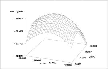
To plot the likelihood surface using the G3D procedure from SAS/GRAPH software, use the following source:
proc g3d data=parms; plot CovP1*CovP2 = ResLogLike / ctop=red cbottom=blue caxis=black; run;
The results from this plot are shown in Output 46.3.2. The peak of the surface is the REML estimates for the B and A * B variance components.
| |
| |
Example 46.4. Known G and R
This animal breeding example from Henderson (1984, p. 53) considers multiple traits. The data are artificial and consist of measurements of two traits on three animals, but the second trait of the third animal is missing. Assuming an additive genetic model, you can use PROC MIXED to predict the breeding value of both traits on all three animals and also to predict the second trait of the third animal. The data are as follows:
data h; input Trait Animal Y; datalines; 1 1 6 1 2 8 1 3 7 2 1 9 2 2 5 2 3 . ;
Both G and R are known.
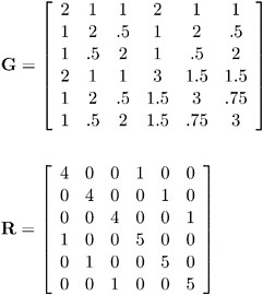
In order to read G into PROC MIXED using the GDATA= option in the RANDOM statement, perform the following DATA step:
data g; input Row Col1-Col6; datalines; 1 2 1 1 2 1 1 2 1 2 .5 1 2 .5 3 1 .5 2 1 .5 2 4 2 1 1 3 1.5 1.5 5 1 2 .5 1.5 3 .75 6 1 .5 2 1.5 .75 3 ;
The preceding data are in the dense representation for a GDATA= data set. You can also construct a data set with the sparse representation using Row , Col ,and Value variables, although this would require 21 observations instead of 6 for this example. The PROC MIXED code is as follows:
proc mixed data=h mmeq mmeqsol; class Trait Animal; model Y = Trait / noint s outp=predicted; random Trait*Animal / type=un gdata=g g gi s; repeated / type=un sub=Animal r ri; parms (4) (1) (5) / noiter; run; proc print data=predicted; run;
The MMEQ and MMEQSOL options request the mixed model equations and their solution. The variables Trait and Animal are classification variables, and Trait defines the entire X matrix for the fixed-effects portion of the model, since the intercept is omitted with the NOINT option. The fixed-effects solution vector and predicted values are also requested using the S and OUTP= options, respectively.
The random effect Trait * Animal leads to a Z matrix with six columns, the first five corresponding to the identity matrix and the last consisting of 0s. An unstructured G matrix is specified using the TYPE=UN option, and it is read into PROC MIXED from a SAS data set using the GDATA=G specification. The G and GI options request the display of G and G ˆ’ 1 , respectively. The S option requests that the random-effects solution vector be displayed.
Note that the preceding R matrix is block diagonal if the data are sorted by animals. The REPEATED statement exploits this fact by requesting R to have unstructured 2 — 2 blocks corresponding to animals, which are the subjects. The R and RI options request that the estimated 2 — 2 blocks for the first animal and its inverse be displayed. The PARMS statement lists the parameters of this 2 — 2 matrix. Note that the parameters from G are not specified in the PARMS statement because they have already been assigned using the GDATA= option in the RANDOM statement. The NOITER option prevents PROC MIXED from computing residual (restricted) maximum likelihood estimates; instead, the known values are used for inferences.
The results from this analysis are shown in Output 46.4.1.
| |
The Mixed Procedure Model Information Data Set WORK.H Dependent Variable Y Covariance Structure Unstructured Subject Effect Animal Estimation Method REML Residual Variance Method None Fixed Effects SE Method Model-Based Degrees of Freedom Method Containment
| |
The Unstructured covariance structure applies to both G and R here.
The Mixed Procedure Class Level Information Class Levels Values Trait 2 1 2 Animal 3 1 2 3
The levels of Trait and Animal have been specified correctly.
The Mixed Procedure Dimensions Covariance Parameters 3 Columns in X 2 Columns in Z 6 Subjects 1 Max Obs Per Subject 6 Number of Observations Number of Observations Read 6 Number of Observations Used 5 Number of Observations Not Used 1
The three covariance parameters indicated here correspond to those from the R matrix. Those from G are considered fixed and known because of the GDATA= option.
The Mixed Procedure Parameter Search CovP1 CovP2 CovP3 Res Log Like -2 Res Log Like 4.0000 1.0000 5.0000 -7.3731 14.7463
The preceding table results from the PARMS statement.
The Mixed Procedure Estimated R Matrix for Subject 1 Row Col1 Col2 1 4.0000 1.0000 2 1.0000 5.0000
The block of R corresponding to the first animal is shown in the Estimated R Matrix table.
The Mixed Procedure Estimated Inv(R) Matrix for Subject 1 Row Col1 Col2 1 0.2632 -0.05263 2 -0.05263 0.2105
The inverse of the block of R corresponding to the first animal is shown in the preceding table.
The Mixed Procedure Estimated G Matrix Row Effect Trait Animal Col1 Col2 Col3 Col4 1 Trait*Animal 1 1 2.0000 1.0000 1.0000 2.0000 2 Trait*Animal 1 2 1.0000 2.0000 0.5000 1.0000 3 Trait*Animal 1 3 1.0000 0.5000 2.0000 1.0000 4 Trait*Animal 2 1 2.0000 1.0000 1.0000 3.0000 5 Trait*Animal 2 2 1.0000 2.0000 0.5000 1.5000 6 Trait*Animal 2 3 1.0000 0.5000 2.0000 1.5000 Estimated G Matrix Row Col5 Col6 1 1.0000 1.0000 2 2.0000 0.5000 3 0.5000 2.0000 4 1.5000 1.5000 5 3.0000 0.7500 6 0.7500 3.0000
The preceding table lists the G matrix as specified in the GDATA= data set.
The Mixed Procedure Estimated Inv(G) Matrix Row Effect Trait Animal Col1 Col2 Col3 Col4 1 Trait*Animal 1 1 2.5000 -1.0000 -1.0000 -1.6667 2 Trait*Animal 1 2 -1.0000 2.0000 0.6667 3 Trait*Animal 1 3 -1.0000 2.0000 0.6667 4 Trait*Animal 2 1 -1.6667 0.6667 0.6667 1.6667 5 Trait*Animal 2 2 0.6667 -1.3333 -0.6667 6 Trait*Animal 2 3 0.6667 -1.3333 -0.6667 Estimated Inv(G) Matrix Row Col5 Col6 1 0.6667 0.6667 2 -1.3333 3 -1.3333 4 -0.6667 -0.6667 5 1.3333 6 1.3333
The preceding table lists G ˆ’ 1 . The blank values correspond to zeros.
The Mixed Procedure Covariance Parameter Estimates Cov Parm Subject Estimate UN(1,1) Animal 4.0000 UN(2,1) Animal 1.0000 UN(2,2) Animal 5.0000
The parameters from R are listed again.
The Mixed Procedure Fit Statistics -2 Res Log Likelihood 14.7 AIC (smaller is better) 14.7 AICC (smaller is better) 14.7 BIC (smaller is better) 14.7
You can use this model-fitting information to compare this model with others.
The Mixed Procedure Mixed Model Equations Row Effect Trait Animal Col1 Col2 Col3 Col4 1 Trait 1 0.7763 -0.1053 0.2632 0.2632 2 Trait 2 -0.1053 0.4211 -0.05263 -0.05263 3 Trait*Animal 1 1 0.2632 -0.05263 2.7632 -1.0000 4 Trait*Animal 1 2 0.2632 -0.05263 -1.0000 2.2632 5 Trait*Animal 1 3 0.2500 -1.0000 6 Trait*Animal 2 1 -0.05263 0.2105 -1.7193 0.6667 7 Trait*Animal 2 2 -0.05263 0.2105 0.6667 -1.3860 8 Trait*Animal 2 3 0.6667 Mixed Model Equations Row Col5 Col6 Col7 Col8 Col9 1 0.2500 -0.05263 -0.05263 4.6974 2 0.2105 0.2105 2.2105 3 -1.0000 -1.7193 0.6667 0.6667 1.1053 4 0.6667 -1.3860 1.8421 5 2.2500 0.6667 -1.3333 1.7500 6 0.6667 1.8772 -0.6667 -0.6667 1.5789 7 -0.6667 1.5439 0.6316 8 -1.3333 -0.6667 1.3333
The coefficients of the mixed model equations agree with Henderson (1984, p. 55).
The Mixed Procedure Mixed Model Equations Solution Row Effect Trait Animal Col1 Col2 Col3 Col4 1 Trait 1 2.5508 1.5685 -1.3047 -1.1775 2 Trait 2 1.5685 4.5539 -1.4112 -1.3534 3 Trait*Animal 1 1 -1.3047 -1.4112 1.8282 1.0652 4 Trait*Animal 1 2 -1.1775 -1.3534 1.0652 1.7589 5 Trait*Animal 1 3 -1.1701 -0.9410 1.0206 0.7085 6 Trait*Animal 2 1 -1.3002 -2.1592 1.8010 1.0900 7 Trait*Animal 2 2 -1.1821 -2.1055 1.0925 1.7341 8 Trait*Animal 2 3 -1.1678 -1.3149 1.0070 0.7209 Mixed Model Equations Solution Row Col5 Col6 Col7 Col8 Col9 1 -1.1701 -1.3002 -1.1821 -1.1678 6.9909 2 -0.9410 -2.1592 -2.1055 -1.3149 6.9959 3 1.0206 1.8010 1.0925 1.0070 0.05450 4 0.7085 1.0900 1.7341 0.7209 -0.04955 5 1.7812 1.0095 0.7197 1.7756 0.02230 6 1.0095 2.7518 1.6392 1.4849 0.2651 7 0.7197 1.6392 2.6874 0.9930 -0.2601 8 1.7756 1.4849 0.9930 2.7645 0.1276
The solution to the mixed model equations also matches that given by Henderson (1984, p. 55).
The Mixed Procedure Solution for Fixed Effects Standard Effect Trait Estimate Error DF t Value Pr > t Trait 1 6.9909 1.5971 3 4.38 0.0221 Trait 2 6.9959 2.1340 3 3.28 0.0465
The estimates for the two traits are nearly identical, but the standard error of the second one is larger because of the missing observation.
The Mixed Procedure Solution for Random Effects Std Err Effect Trait Animal Estimate Pred DF t Value Pr > t Trait*Animal 1 1 0.05450 1.3521 0 0.04 . Trait*Animal 1 2 -0.04955 1.3262 0 -0.04 . Trait*Animal 1 3 0.02230 1.3346 0 0.02 . Trait*Animal 2 1 0.2651 1.6589 0 0.16 . Trait*Animal 2 2 -0.2601 1.6393 0 -0.16 . Trait*Animal 2 3 0.1276 1.6627 0 0.08 .
The Estimate column lists the best linear unbiased predictions (BLUPs) of the breeding values of both traits for all three animals. The p -values are missing because the default containment method for computing degrees of freedom results in zero degrees of freedom for the random effects parameter tests.
The Mixed Procedure Type 3 Tests of Fixed Effects Num Den Effect DF DF F Value Pr > F Trait 2 3 10.59 0.0437
The two estimated traits are significantly different from zero at the 5% level.
StdErr Obs Trait Animal Y Pred Pred DF Alpha Lower Upper Resid 1 1 1 6 7.04542 1.33027 0 0.05 . . -1.04542 2 1 2 8 6.94137 1.39806 0 0.05 . . 1.05863 3 1 3 7 7.01321 1.41129 0 0.05 . . -0.01321 4 2 1 9 7.26094 1.72839 0 0.05 . . 1.73906 5 2 2 5 6.73576 1.74077 0 0.05 . . -1.73576 6 2 3 . 7.12015 2.99088 0 0.05 . . .
The preceding table contains the predicted values of the observations based on the trait and breeding value estimates, that is, the fixed and random effects. The predicted values are not the predictions of future records in the sense that they do not contain a component corresponding to a new observational error. Refer to Henderson (1984) for information on predicting future records. The L95 and U95 columns usually contain confidence limits for the predicted values; they are missing here because the random-effects parameter degrees of freedom equals 0.
Example 46.5. Random Coefficients
This example comes from a pharmaceutical stability data simulation performed by Obenchain (1990). The observed responses are replicate assay results, expressed in percent of label claim, at various shelf ages, expressed in months. The desired mixed model involves three batches of product that differ randomly in intercept (initial potency) and slope (degradation rate). This type of model is also known as a hierarchical or multilevel model (Singer 1998; Sullivan, Dukes, and Losina 1999).
The SAS code is as follows:
data rc; input Batch Month @@; Monthc = Month; do i = 1 to 6; input Y @@; output; end; datalines; 1 0 101.2 103.3 103.3 102.1 104.4 102.4 1 1 98.8 99.4 99.7 99.5 . . 1 3 98.4 99.0 97.3 99.8 . . 1 6 101.5 100.2 101.7 102.7 . . 1 9 96.3 97.2 97.2 96.3 . . 1 12 97.3 97.9 96.8 97.7 97.7 96.7 2 0 102.6 102.7 102.4 102.1 102.9 102.6 2 1 99.1 99.0 99.9 100.6 . . 2 3 105.7 103.3 103.4 104.0 . . 2 6 101.3 101.5 100.9 101.4 . . 2 9 94.1 96.5 97.2 95.6 . . 2 12 93.1 92.8 95.4 92.2 92.2 93.0 3 0 105.1 103.9 106.1 104.1 103.7 104.6 3 1 102.2 102.0 100.8 99.8 . . 3 3 101.2 101.8 100.8 102.6 . . 3 6 101.1 102.0 100.1 100.2 . . 3 9 100.9 99.5 102.2 100.8 . . 3 12 97.8 98.3 96.9 98.4 96.9 96.5 ; proc mixed data=rc; class Batch; model Y = Month / s; random Int Month / type=un sub=Batch s; run;
In the DATA step, Monthc is created as a duplicate of Month in order to enable both a continuous and classification version of the same variable. The variable Monthc is used in a subsequent analysis on page 2814.
In the PROC MIXED code, Batch is listed as the only classification variable. The fixed effect Month in the MODEL statement is not declared a classification variable; thus it models a linear trend in time. An intercept is included as a fixed effect by default, and the S option requests that the fixed-effects parameter estimates be produced.
The two RANDOM effects are Int and Month , modeling random intercepts and slopes, respectively. Note that Intercept and Month are used as both fixed and random effects. The TYPE=UN option in the RANDOM statement specifies an unstructured covariance matrix for the random intercept and slope effects. In mixed model notation, G is block diagonal with unstructured 2 — 2 blocks. Each block corresponds to a different level of Batch , which is the SUBJECT= effect. The unstructured type provides a mechanism for estimating the correlation between the random coefficients. The S option requests the production of the random-effects parameter estimates.
The results from this analysis are shown in Output 46.5.1.
| |
The Mixed Procedure Model Information Data Set WORK.RC Dependent Variable Y Covariance Structure Unstructured Subject Effect Batch Estimation Method REML Residual Variance Method Profile Fixed Effects SE Method Model-Based Degrees of Freedom Method Containment
| |
The Unstructured covariance structure applies to G here.
The Mixed Procedure Class Level Information Class Levels Values Batch 3 1 2 3
Batch is the only classification variable in this analysis, and it has three levels.
The Mixed Procedure Dimensions Covariance Parameters 4 Columns in X 2 Columns in Z Per Subject 2 Subjects 3 Max Obs Per Subject 36 Number of Observations Number of Observations Read 108 Number of Observations Used 84 Number of Observations Not Used 24
The Dimensions table indicates that there are three subjects (corresponding to batches). The 24 observations not used correspond to the missing values of Y in the input data set.
The Mixed Procedure Iteration History Iteration Evaluations -2 Res Log Like Criterion 0 1 367.02768461 1 1 350.32813577 0.00000000 Convergence criteria met.
Only one iteration is required for convergence.
The Mixed Procedure Covariance Parameter Estimates Cov Parm Subject Estimate UN(1,1) Batch 0.9768 UN(2,1) Batch -0.1045 UN(2,2) Batch 0.03717 Residual 3.2932
The estimated elements of the unstructured 2 — 2 matrix comprising the blocks of G are listed in the Estimate column. Note that the random coefficients are negatively correlated.
The Mixed Procedure Fit Statistics -2 Res Log Likelihood 350.3 AIC (smaller is better) 358.3 AICC (smaller is better) 358.8 BIC (smaller is better) 354.7 Null Model Likelihood Ratio Test DF Chi-Square Pr > ChiSq 3 16.70 0.0008
The null model likelihood ratio test indicates a significant improvement over the null model consisting of no random effects and a homogeneous residual error.
The Mixed Procedure Solution for Fixed Effects Standard Effect Estimate Error DF t Value Pr > t Intercept 102.70 0.6456 2 159.08 <.0001 Month -0.5259 0.1194 2 -4.41 0.0478
The fixed effects estimates represent the estimated means for the random intercept and slope, respectively.
The Mixed Procedure Solution for Random Effects Std Err Effect Batch Estimate Pred DF t Value Pr > t Intercept 1 -1.0010 0.6842 78 -1.46 0.1474 Month 1 0.1287 0.1245 78 1.03 0.3047 Intercept 2 0.3934 0.6842 78 0.58 0.5669 Month 2 -0.2060 0.1245 78 -1.65 0.1021 Intercept 3 0.6076 0.6842 78 0.89 0.3772 Month 3 0.07731 0.1245 78 0.62 0.5365
The random effects estimates represent the estimated deviation from the mean intercept and slope for each batch. Therefore, the intercept for the first batch is close to 102 . 7 ˆ’ 1 = 101 . 7, while the intercepts for the other two batches are greater than 102.7. The second batch has a slope less than the mean slope of ˆ’ . 526, while the other two batches have slopes larger than ˆ’ . 526.
The Mixed Procedure Type 3 Tests of Fixed Effects Num Den Effect DF DF F Value Pr > F Month 1 2 19.41 0.0478
The F -statistic in the Type 3 Tests of Fixed Effects table is the square of the t -statistic used in the test of Month in the preceding Solution for Fixed Effects table. Both statistics test the null hypothesis that the slope assigned to Month equals 0, and this hypothesis can barely be rejected at the 5% level.
It is also possible to fit a random coefficients model with error terms that follow a nested structure (Fuller and Battese 1973). The following SAS code represents one way of doing this:
proc mixed data=rc; class Batch Monthc; model Y = Month / s; random Int Month Monthc / sub=Batch s; run;
The variable Monthc is added to the CLASS and RANDOM statements, and it models the nested errors. Note that Month and Monthc are continuous and classification versions of the same variable. Also, the TYPE=UN option is dropped from the RANDOM statement, resulting in the default variance components model instead of correlated random coefficients.
The results from this analysis are shown in Output 46.5.2.
| |
The Mixed Procedure Model Information Data Set WORK.RC Dependent Variable Y Covariance Structure Variance Components Subject Effect Batch Estimation Method REML Residual Variance Method Profile Fixed Effects SE Method Model-Based Degrees of Freedom Method Containment Class Level Information Class Levels Values Batch 3 1 2 3 Monthc 6 0 1 3 6 9 12 Dimensions Covariance Parameters 4 Columns in X 2 Columns in Z Per Subject 8 Subjects 3 Max Obs Per Subject 36 Number of Observations Number of Observations Read 108 Number of Observations Used 84 Number of Observations Not Used 24 Iteration History Iteration Evaluations -2 Res Log Like Criterion 0 1 367.02768461 1 4 277.51945360 . 2 1 276.97551718 0.00104208 3 1 276.90304909 0.00003174 4 1 276.90100316 0.00000004 5 1 276.90100092 0.00000000 Convergence criteria met. Covariance Parameter Estimates Cov Parm Subject Estimate Intercept Batch 0 Month Batch 0.01243 Monthc Batch 3.7411 Residual 0.7969
| |
For this analysis, the Newton-Raphson algorithm requires five iterations and nine likelihood evaluations to achieve convergence. The missing value in the Criterion column in iteration 1 indicates that a boundary constraint has been dropped.
The estimate for the Intercept variance component equals 0. This occurs frequently in practice and indicates that the restricted likelihood is maximized by setting this variance component equal to 0. Whenever a zero variance component estimate occurs, the following note appears in the SAS log:
NOTE: Estimated G matrix is not positive definite.
The remaining variance component estimates are positive, and the estimate corresponding to the nested errors (MONTHC) is much larger than the other two.
The Mixed Procedure Fit Statistics -2 Res Log Likelihood 276.9 AIC (smaller is better) 282.9 AICC (smaller is better) 283.2 BIC (smaller is better) 280.2
A comparison of AIC and BIC for this model with those of the previous model favors the nested error model. Strictly speaking, a likelihood ratio test cannot be carried out between the two models because one is not contained in the other; however, a cautious comparison of likelihoods can be informative.
The Mixed Procedure Solution for Fixed Effects Standard Effect Estimate Error DF t Value Pr > t Intercept 102.56 0.7287 2 140.74 <.0001 Month -0.5003 0.1259 2 -3.97 0.0579
The better-fitting covariance model impacts the standard errors of the fixed effects parameter estimates more than the estimates themselves .
The Mixed Procedure Solution for Random Effects Std Err Effect Batch Monthc Estimate Pred DF t Value Pr > t Intercept 1 0 . . . . Month 1 -0.00028 0.09268 66 -0.00 0.9976 Monthc 1 0 0.2191 0.7896 66 0.28 0.7823 Monthc 1 1 -2.5690 0.7571 66 -3.39 0.0012 Monthc 1 3 -2.3067 0.6865 66 -3.36 0.0013 Monthc 1 6 1.8726 0.7328 66 2.56 0.0129 Monthc 1 9 -1.2350 0.9300 66 -1.33 0.1888 Monthc 1 12 0.7736 1.1992 66 0.65 0.5211 Intercept 2 0 . . . . Month 2 -0.07571 0.09268 66 -0.82 0.4169 Monthc 2 0 -0.00621 0.7896 66 -0.01 0.9938 Monthc 2 1 -2.2126 0.7571 66 -2.92 0.0048 Monthc 2 3 3.1063 0.6865 66 4.53 <.0001 Monthc 2 6 2.0649 0.7328 66 2.82 0.0064 Monthc 2 9 -1.4450 0.9300 66 -1.55 0.1250 Monthc 2 12 -2.4405 1.1992 66 -2.04 0.0459 Intercept 3 0 . . . . Month 3 0.07600 0.09268 66 0.82 0.4152 Monthc 3 0 1.9574 0.7896 66 2.48 0.0157 Monthc 3 1 -0.8850 0.7571 66 -1.17 0.2466 Monthc 3 3 0.3006 0.6865 66 0.44 0.6629 Monthc 3 6 0.7972 0.7328 66 1.09 0.2806 Monthc 3 9 2.0059 0.9300 66 2.16 0.0347
The random effects solution provides the empirical best linear unbiased predictions (EBLUPs) for the realizations of the random intercept, slope, and nested errors. You can use these values to compare batches and months.
The Mixed Procedure Type 3 Tests of Fixed Effects Num Den Effect DF DF F Value Pr > F Month 1 2 15.78 0.0579
The test of Month is similar to that from the previous model, although it is no longer significant at the 5% level.
Example 46.6. Line-Source Sprinkler Irrigation
These data appear in Hanks et al. (1980), Johnson, Chaudhuri, and Kanemasu (1983), and Stroup (1989b). Three cultivars ( Cult ) of winter wheat are randomly assigned to rectangular plots within each of three blocks ( Block ). The nine plots are located side-by-side, and a line-source sprinkler is placed through the middle. Each plot is subdivided into twelve subplots, six to the north of the line-source, six to the south ( Dir ). The two plots closest to the line-source represent the maximum irrigation level ( Irrig =6), the two next-closest plots represent the next -highest level ( Irrig =5), and so forth.
This example is a case where both G and R can be modeled . One of Stroup s models specifies a diagonal G containing the variance components for Block , Block * Dir , and Block * Irrig , and a Toeplitz R with four bands. The SAS code to fit this model and carry out some further analyses follows.
Caution: This analysis may require considerable CPU time.
data line; length Cult$ 8; input Block Cult$ @; row = _n_; do Sbplt=1 to 12; if Sbplt le 6 then do; Irrig = Sbplt; Dir = North; end; else do; Irrig = 13 - Sbplt; Dir = South; end; input Y @; output; end; datalines; 1 Luke 2.4 2.7 5.6 7.5 7.9 7.1 6.1 7.3 7.4 6.7 3.8 1.8 1 Nugaines 2.2 2.2 4.3 6.3 7.9 7.1 6.2 5.3 5.3 5.2 5.4 2.9 1 Bridger 2.9 3.2 5.1 6.9 6.1 7.5 5.6 6.5 6.6 5.3 4.1 3.1 2 Nugaines 2.4 2.2 4.0 5.8 6.1 6.2 7.0 6.4 6.7 6.4 3.7 2.2 2 Bridger 2.6 3.1 5.7 6.4 7.7 6.8 6.3 6.2 6.6 6.5 4.2 2.7 2 Luke 2.2 2.7 4.3 6.9 6.8 8.0 6.5 7.3 5.9 6.6 3.0 2.0 3 Nugaines 1.8 1.9 3.7 4.9 5.4 5.1 5.7 5.0 5.6 5.1 4.2 2.2 3 Luke 2.1 2.3 3.7 5.8 6.3 6.3 6.5 5.7 5.8 4.5 2.7 2.3 3 Bridger 2.7 2.8 4.0 5.0 5.2 5.2 5.9 6.1 6.0 4.3 3.1 3.1 ; proc mixed; class Block Cult Dir Irrig; model Y = CultDirIrrig@2; random Block Block*Dir Block*Irrig; repeated / type=toep(4) sub=Block*Cult r; lsmeans CultIrrig; estimate Bridger vs Luke Cult 1 -1 0; estimate Linear Irrig Irrig -5 -3 -1 1 3 5; estimate B vs L x Linear Irrig Cult*Irrig -5 -3 -1 1 3 5 5 3 1 -1 -3 -5; run;
The preceding code uses the bar operator ()and the at sign (@) to specify all two-factor interactions between Cult , Dir ,and Irrig as fixed effects.
The RANDOM statement sets up the Z and G matrices corresponding to the random effects Block , Block * Dir ,and Block * Irrig .
In the REPEATED statement, the TYPE=TOEP(4) option sets up the blocks of the R matrix to be Toeplitz with four bands below and including the main diagonal. The subject effect is Block ( Cult ), and it produces nine 12 — 12 blocks. The R option requests that the first block of R be displayed.
Least-squares means (LSMEANS) are requested for Cult , Irrig , and Cult * Irrig , and a few ESTIMATE statements are specified to illustrate some linear combinations of the fixed effects.
The results from this analysis are shown in Output 46.6.1.
| |
The Mixed Procedure Model Information Data Set WORK.LINE Dependent Variable Y Covariance Structures Variance Components, Toeplitz Subject Effect Block*Cult Estimation Method REML Residual Variance Method Profile Fixed Effects SE Method Model-Based Degrees of Freedom Method Containment
| |
The Covariance Structures row reveals the two different structures assumed for G and R .
The Mixed Procedure Class Level Information Class Levels Values Block 3 1 2 3 Cult 3 Bridger Luke Nugaines Dir 2 North South Irrig 6 1 2 3 4 5 6
The levels of each class variable are listed as a single string in the Values column, regardless of whether the levels are numeric or character.
The Mixed Procedure Dimensions Covariance Parameters 7 Columns in X 48 Columns in Z 27 Subjects 1 Max Obs Per Subject 108 Number of Observations Number of Observations Read 108 Number of Observations Used 108 Number of Observations Not Used 0
Even though there is a SUBJECT= effect in the REPEATED statement, the analysis considers all of the data to be from one subject because there is no corresponding SUBJECT= effect in the RANDOM statement.
The Mixed Procedure Iteration History Iteration Evaluations -2 Res Log Like Criterion 0 1 226.25427252 1 4 187.99336173 . 2 3 186.62579299 0.10431081 3 1 184.38218213 0.04807260 4 1 183.41836853 0.00886548 5 1 183.25111475 0.00075353 6 1 183.23809997 0.00000748 7 1 183.23797748 0.00000000 Convergence criteria met.
The Newton-Raphson algorithm converges successfully in seven iterations.
The Mixed Procedure Estimated R Matrix for Subject 1 Row Col1 Col2 Col3 Col4 Col5 Col6 Col7 1 0.2850 0.007986 0.001452 -0.09253 2 0.007986 0.2850 0.007986 0.001452 -0.09253 3 0.001452 0.007986 0.2850 0.007986 0.001452 -0.09253 4 -0.09253 0.001452 0.007986 0.2850 0.007986 0.001452 -0.09253 5 -0.09253 0.001452 0.007986 0.2850 0.007986 0.001452 6 -0.09253 0.001452 0.007986 0.2850 0.007986 7 -0.09253 0.001452 0.007986 0.2850 8 -0.09253 0.001452 0.007986 9 -0.09253 0.001452 10 -0.09253 11 12 Estimated R Matrix for Subject 1 Row Col8 Col9 Col10 Col11 Col12 1 2 3 4 5 -0.09253 6 0.001452 -0.09253 7 0.007986 0.001452 -0.09253 8 0.2850 0.007986 0.001452 -0.09253 9 0.007986 0.2850 0.007986 0.001452 -0.09253 10 0.001452 0.007986 0.2850 0.007986 0.001452 11 -0.09253 0.001452 0.007986 0.2850 0.007986 12 -0.09253 0.001452 0.007986 0.2850
The first block of the estimated R matrix has the TOEP(4) structure, and the observations that are three plots apart exhibit a negative correlation.
The Mixed Procedure Covariance Parameter Estimates Cov Parm Subject Estimate Block 0.2194 Block*Dir 0.01768 Block*Irrig 0.03539 TOEP(2) Block*Cult 0.007986 TOEP(3) Block*Cult 0.001452 TOEP(4) Block*Cult -0.09253 Residual 0.2850
The preceding table lists the estimated covariance parameters from both G and R . The first three are the variance components making up the diagonal G , and the final four make up the Toeplitz structure in the blocks of R . The Residual row corresponds to the variance of the Toeplitz structure, and it was the parameter profiled out during the optimization process.
The Mixed Procedure Fit Statistics -2 Res Log Likelihood 183.2 AIC (smaller is better) 197.2 AICC (smaller is better) 198.8 BIC (smaller is better) 190.9
The ˆ’ 2 Res Log Likelihood value is the same as the final value listed in the Iteration History table.
The Mixed Procedure Type 3 Tests of Fixed Effects Num Den Effect DF DF F Value Pr > F Cult 2 68 7.98 0.0008 Dir 1 2 3.95 0.1852 Cult*Dir 2 68 3.44 0.0379 Irrig 5 10 102.60 <.0001 Cult*Irrig 10 68 1.91 0.0580 Dir*Irrig 5 68 6.12 <.0001
Every fixed effect except for Dir and Cult * Irrig is significant at the 5% level.
The Mixed Procedure Estimates Standard Label Estimate Error DF t Value Pr > t Bridger vs Luke -0.03889 0.09524 68 -0.41 0.6843 Linear Irrig 30.6444 1.4412 10 21.26 <.0001 B vs L x Linear Irrig -9.8667 2.7400 68 -3.60 0.0006
The Estimates table lists the results from the various linear combinations of fixed effects specified in the ESTIMATE statements. Bridger is not significantly different from Luke, and Irrig possesses a strong linear component. This strength appears to be influencing the significance of the interaction.
The Mixed Procedure Least Squares Means Standard Effect Cult Irrig Estimate Error DF t Value Pr > t Cult Bridger 5.0306 0.2874 68 17.51 <.0001 Cult Luke 5.0694 0.2874 68 17.64 <.0001 Cult Nugaines 4.7222 0.2874 68 16.43 <.0001 Irrig 1 2.4222 0.3220 10 7.52 <.0001 Irrig 2 3.1833 0.3220 10 9.88 <.0001 Irrig 3 5.0556 0.3220 10 15.70 <.0001 Irrig 4 6.1889 0.3220 10 19.22 <.0001 Irrig 5 6.4000 0.3140 10 20.38 <.0001 Irrig 6 6.3944 0.3227 10 19.81 <.0001 Cult*Irrig Bridger 1 2.8500 0.3679 68 7.75 <.0001 Cult*Irrig Bridger 2 3.4167 0.3679 68 9.29 <.0001 Cult*Irrig Bridger 3 5.1500 0.3679 68 14.00 <.0001 Cult*Irrig Bridger 4 6.2500 0.3679 68 16.99 <.0001 Cult*Irrig Bridger 5 6.3000 0.3463 68 18.19 <.0001 Cult*Irrig Bridger 6 6.2167 0.3697 68 16.81 <.0001 Cult*Irrig Luke 1 2.1333 0.3679 68 5.80 <.0001 Cult*Irrig Luke 2 2.8667 0.3679 68 7.79 <.0001 Cult*Irrig Luke 3 5.2333 0.3679 68 14.22 <.0001 Cult*Irrig Luke 4 6.5500 0.3679 68 17.80 <.0001 Cult*Irrig Luke 5 6.8833 0.3463 68 19.87 <.0001 Cult*Irrig Luke 6 6.7500 0.3697 68 18.26 <.0001 Cult*Irrig Nugaines 1 2.2833 0.3679 68 6.21 <.0001 Cult*Irrig Nugaines 2 3.2667 0.3679 68 8.88 <.0001 Cult*Irrig Nugaines 3 4.7833 0.3679 68 13.00 <.0001 Cult*Irrig Nugaines 4 5.7667 0.3679 68 15.67 <.0001 Cult*Irrig Nugaines 5 6.0167 0.3463 68 17.37 <.0001 Cult*Irrig Nugaines 6 6.2167 0.3697 68 16.81 <.0001
The LS-means are useful in comparing the levels of the various fixed effects. For example, it appears that irrigation levels 5 and 6 have virtually the same effect.
An interesting exercise is to try fitting other variance-covariance models to these data and comparing them to this one using likelihood ratio tests, Akaike s Information Criterion, or Schwarz s Bayesian Information Criterion. In particular, some spatial models are worth investigating (Marx and Thompson 1987; Zimmerman and Harville 1991). The following is one example of spatial model code.
proc mixed; class Block Cult Dir Irrig; model Y = CultDirIrrig@2; repeated / type=sp(pow)(Row Sbplt) sub=intercept; run;
The TYPE=SP(POW)(ROW SBPLT) option in the REPEATED statement requests the spatial power structure, with the two defining coordinate variables being Row and Sbplt . The SUB=INTERCEPT option indicates that the entire data set is to be considered as one subject, thereby modeling R as a dense 108 — 108 covariance matrix. Refer to Wolfinger (1993) for further discussion of this example and additional analyses.
Example 46.7. Influence in Heterogeneous Variance Model (Experimental)
In this example from Snedecor and Cochran (1976, p. 256) a one-way classification model with heterogeneous variances is fit. The data represent amounts of different types of fat absorbed by batches of doughnuts during cooking, measured in grams.
data absorb; input FatType Absorbed @@; datalines; 1 164 1 172 1 168 1 177 1 156 1 195 2 178 2 191 2 197 2 182 2 185 2 177 3 175 3 193 3 178 3 171 3 163 3 176 4 155 4 166 4 149 4 164 4 170 4 168 ;
The statistical model for these data can be written as
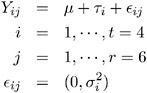
where Y ij is the amount of fat absorbed by the j th batch of the i th fat type, and i denotes the fat-type effects. A quick glance at the data suggests that observations 6, 9, 14, and 21 might be influential on the analysis, because these are extreme observations for the respective fat types.
The following SAS statements fit this model and request influence diagnostics for the fixed effects and covariance parameters. The experimental ODS GRAPHICS statement requests plots of the influence diagnostics in addition to the tabular output. The ESTIMATE suboption requests plots of leave-one-out estimates for the fixed effects and group variances.
ods html; ods graphics on; proc mixed data=absorb asycov; class FatType; model Absorbed = FatType / s influence(iter=10 estimates); repeated / group=FatType; ods output Influence=inf; run; ods graphics off; ods html close;
The Influence table is output to the SAS data set inf so that parameter estimates can be printed subsequently. Results from this analysis are shown in Output 46.7.1.
| |
The Mixed Procedure Model Information Data Set WORK.ABSORB Dependent Variable Absorbed Covariance Structure Variance Components Group Effect FatType Estimation Method REML Residual Variance Method None Fixed Effects SE Method Model-Based Degrees of Freedom Method Between-Within Covariance Parameter Estimates Cov Parm Group Estimate Residual FatType 1 178.00 Residual FatType 2 60.4000 Residual FatType 3 97.6000 Residual FatType 4 67.6000 Solution for Fixed Effects Fat Standard Effect Type Estimate Error DF t Value Pr > t Intercept 162.00 3.3566 20 48.26 <.0001 FatType 1 10.0000 6.3979 20 1.56 0.1337 FatType 2 23.0000 4.6188 20 4.98 <.0001 FatType 3 14.0000 5.2472 20 2.67 0.0148 FatType 4 0 . . . .
| |
The variances in the four groups are shown in the Covariance Parameter Estimates table. The estimated variance in the first group is two to three times larger than the variance in the other groups.
The fixed effects solutions correspond to estimates of the following parameters:
Intercept : ¼ + 4
FatType 1 : 1 ˆ’ 4
FatType 2 : 2 ˆ’ 4
FatType 3 : 3 ˆ’ 4
FatType 4 : 0
You can easily verify that these estimates are simple functions of the arithmetic means y i. in the groups. For example, ![]() , and so forth. The covariance parameter estimates are the sample variances in the groups and are uncorrelated.
, and so forth. The covariance parameter estimates are the sample variances in the groups and are uncorrelated.
The Mixed Procedure Asymptotic Covariance Matrix of Estimates Row Cov Parm CovP1 CovP2 CovP3 CovP4 1 Residual 12674 2 Residual 1459.26 3 Residual 3810.30 4 Residual 1827.90
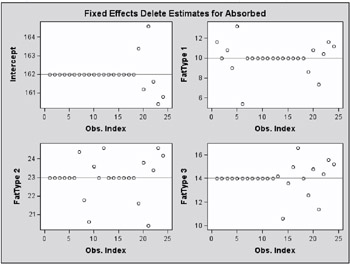
The following statements print the leave-one-out estimates for fixed effects and covariance parameters that were written to the inf data set with the ESTIMATES suboption.
proc print data=inf label; var parm1-parm5 covp1-covp4; run;
| |
Residual Residual Residual Residual Fat Fat Fat Fat FatType FatType FatType FatType Obs Intercept Type 1 Type 2 Type 3 Type 4 1 2 3 4 1 162.00 11.600 23.000 14.000 0 203.30 60.400 97.60 67.600 2 162.00 10.000 23.000 14.000 0 222.47 60.400 97.60 67.600 3 162.00 10.800 23.000 14.000 0 217.68 60.400 97.60 67.600 4 162.00 9.000 23.000 14.000 0 214.99 60.400 97.60 67.600 5 162.00 13.200 23.000 14.000 0 145.70 60.400 97.60 67.600 6 162.00 5.400 23.000 14.000 0 63.80 60.400 97.60 67.600 7 162.00 10.000 24.400 14.000 0 178.00 60.795 97.60 67.600 8 162.00 10.000 21.800 14.000 0 178.00 64.691 97.60 67.600 9 162.00 10.000 20.600 14.000 0 178.00 32.296 97.60 67.600 10 162.00 10.000 23.600 14.000 0 178.00 72.797 97.60 67.600 11 162.00 10.000 23.000 14.000 0 178.00 75.490 97.60 67.600 12 162.00 10.000 24.600 14.000 0 178.00 56.285 97.60 67.600 13 162.00 10.000 23.000 14.200 0 178.00 60.400 121.68 67.600 14 162.00 10.000 23.000 10.600 0 178.00 60.400 35.30 67.600 15 162.00 10.000 23.000 13.600 0 178.00 60.400 120.79 67.600 16 162.00 10.000 23.000 15.000 0 178.00 60.400 114.50 67.600 17 162.00 10.000 23.000 16.600 0 178.00 60.400 71.30 67.600 18 162.00 10.000 23.000 14.000 0 178.00 60.400 121.98 67.600 19 163.40 8.600 21.600 12.600 0 178.00 60.400 97.60 69.799 20 161.20 10.800 23.800 14.800 0 178.00 60.400 97.60 79.698 21 164.60 7.400 20.400 11.400 0 178.00 60.400 97.60 33.800 22 161.60 10.400 23.400 14.400 0 178.00 60.400 97.60 83.292 23 160.40 11.600 24.600 15.600 0 178.00 60.400 97.60 65.299 24 160.80 11.200 24.200 15.200 0 178.00 60.400 97.60 73.677
| |
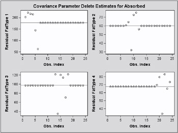
The estimate of the intercept is affected only when observations from the last group are removed. The estimate of the FatType 1 effect reacts to removal of observations in the first and last group (Output 46.7.3).
While observations can impact one or more fixed effects solutions in this model, they can only affect one covariance parameter, the variance in their group (Output 46.7.4). Observations 6, 9, 14, and 21, which are extreme in their group, reduce the group variance considerably.
These graphical displays are requested by specifying the experimental ODS GRAPHICS statement. For general information about ODS graphics, see Chapter 15, Statistical Graphics Using ODS. For specific information about the graphics available in the MIXED procedure, see the ODS Graphics section on page 2757.
| |
| |
| |
| |
Diagnostics related to residuals and predicted values are printed with the following statements.
proc print data=inf label; var observed predicted residual pressres student Rstudent; run;
Observations 6, 9, 14, and 21 have large studentized residuals (Output 46.7.5). That the externally studentized residuals are much larger than the internally studentized residuals for these observations indicates that the variance estimate in the group shrinks when the observation is removed. Also important to note is that comparisons based on raw residuals in models with heterogeneous variance can be misleading. Observation 5, for example, has a larger residual but a smaller studentized residual than observation 21. The variance for the first fat type is much larger than the variance in the fourth group. A large residual is more surprising in the groups with small variance.
| |
Internally Externally Observed Predicted PRESS Studentized Studentized Obs Value Mean Residual Residual Residual Residual 1 164.000 172.000 8.000 9.600 0.6569 0.6146 2 172.000 172.000 0.000 0.000 0.0000 0.0000 3 168.000 172.000 4.000 4.800 0.3284 0.2970 4 177.000 172.000 5.000 6.000 0.4105 0.3736 5 156.000 172.000 16.000 19.200 1.3137 1.4521 6 195.000 172.000 23.000 27.600 1.8885 3.1544 7 178.000 185.000 7.000 8.400 0.9867 0.9835 8 191.000 185.000 6.000 7.200 0.8457 0.8172 9 197.000 185.000 12.000 14.400 1.6914 2.3131 10 182.000 185.000 3.000 3.600 0.4229 0.3852 11 185.000 185.000 0.000 -0.000 0.0000 0.0000 12 177.000 185.000 8.000 9.600 1.1276 1.1681 13 175.000 176.000 1.000 1.200 0.1109 0.0993 14 193.000 176.000 17.000 20.400 1.8850 3.1344 15 178.000 176.000 2.000 2.400 0.2218 0.1993 16 171.000 176.000 5.000 6.000 0.5544 0.5119 17 163.000 176.000 13.000 15.600 1.4415 1.6865 18 176.000 176.000 0.000 0.000 0.0000 0.0000 19 155.000 162.000 7.000 8.400 0.9326 0.9178 20 166.000 162.000 4.000 4.800 0.5329 0.4908 21 149.000 162.000 13.000 15.600 1.7321 2.4495 22 164.000 162.000 2.000 2.400 0.2665 0.2401 23 170.000 162.000 8.000 9.600 1.0659 1.0845 24 168.000 162.000 6.000 7.200 0.7994 0.7657
| |
Diagnostics related to the fixed effects estimates, their precision, and the overall influence on the analysis (likelihood distance) are printed with the following statements.
proc print data=inf label; var leverage observed CookD DFFITS CovRatio RLD; run;
| |
Restr. Observed Cooks Likelihood Obs Leverage Value D DFFITS COVRATIO Distance 1 0.16667 164.000 0.02157 -0.27487 1.3706 0.1178 2 0.16667 172.000 0.00000 0.00000 1.4998 0.1156 3 0.16667 168.000 0.00539 -0.13282 1.4675 0.1124 4 0.16667 177.000 0.00843 0.16706 1.4494 0.1117 5 0.16667 156.000 0.08629 -0.64938 0.9822 0.5290 6 0.16667 195.000 0.17831 1.41069 0.4301 5.8101 7 0.16667 178.000 0.04868 -0.43982 1.2078 0.1935 8 0.16667 191.000 0.03576 0.36546 1.2853 0.1451 9 0.16667 197.000 0.14305 1.03446 0.6416 2.2909 10 0.16667 182.000 0.00894 -0.17225 1.4463 0.1116 11 0.16667 185.000 0.00000 -0.00000 1.4998 0.1156 12 0.16667 177.000 0.06358 -0.52239 1.1183 0.2856 13 0.16667 175.000 0.00061 -0.04441 1.4961 0.1151 14 0.16667 193.000 0.17766 1.40175 0.4340 5.7044 15 0.16667 178.000 0.00246 0.08915 1.4851 0.1139 16 0.16667 171.000 0.01537 -0.22892 1.4078 0.1129 17 0.16667 163.000 0.10389 -0.75423 0.8766 0.8433 18 0.16667 176.000 0.00000 0.00000 1.4998 0.1156 19 0.16667 155.000 0.04349 -0.41047 1.2390 0.1710 20 0.16667 166.000 0.01420 0.21950 1.4148 0.1124 21 0.16667 149.000 0.15000 -1.09545 0.6000 2.7343 22 0.16667 164.000 0.00355 0.10736 1.4786 0.1133 23 0.16667 170.000 0.05680 0.48500 1.1592 0.2383 24 0.16667 168.000 0.03195 0.34245 1.3079 0.1353
| |
| |
| |
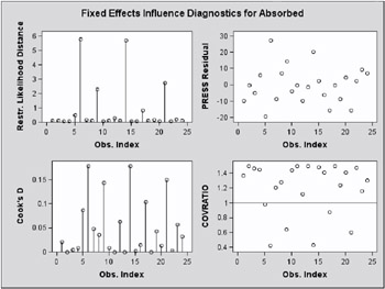
Scanning the restricted likelihood distances, observations 6, 9, 14, and 21 clearly displace the REML solution more than any other observations (Output 46.7.6, Output 46.7.7). These observations are also associated with large values for Cook s D and values of COVRATIO far less than one. The latter indicates that the fixed effects are estimated more precisely when these observations are removed from the analysis.
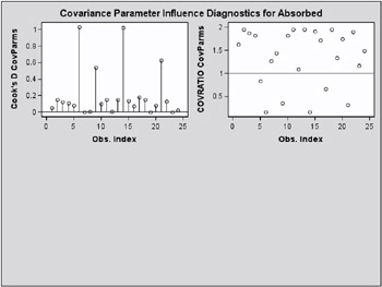
The same conclusions hold for the covariance parameter estimates.
proc print data=inf label; var iter CookDCP CovRatioCP; run;
Observations 6, 9, 14, and 21 change the estimates and their precision considerably (Output 46.7.8, Output 46.7.9). All iterative updates converged within at most four iterations.
| |
Cook s D COVRATIO Obs Iterations CovParms CovParms 1 3 0.05050 1.6306 2 3 0.15603 1.9520 3 3 0.12426 1.8692 4 3 0.10796 1.8233 5 4 0.08232 0.8375 6 4 1.02909 0.1606 7 1 0.00011 1.2662 8 2 0.01262 1.4335 9 3 0.54126 0.3573 10 3 0.10531 1.8156 11 3 0.15603 1.9520 12 2 0.01160 1.0849 13 3 0.15223 1.9425 14 4 1.01865 0.1635 15 3 0.14111 1.9141 16 3 0.07494 1.7203 17 3 0.18154 0.6671 18 3 0.15603 1.9520 19 2 0.00265 1.3326 20 3 0.08008 1.7374 21 1 0.62500 0.3125 22 3 0.13472 1.8974 23 2 0.00290 1.1663 24 2 0.02020 1.4839 | |
| |
| |
Example 46.8. Influence Analysis for Repeated Measures Data (Experimental)
This example revisits the repeated measures data analyzed in Example 46.2. Recall that the data consist of growth measurements at ages 8, 10, 12, and 14 for 11 girls and 16 boys. The model being fit contains fixed effects for Gender , Age and their interaction.
The earlier analysis of these data indicated some unusual observations in this data set. Because of the clustered data structure it is of interest to study the influence of clusters (children) on the analysis rather than the influence of individual observations. A cluster comprises the repeated measurements for each child.
The repeated measures are first modeled with an unstructured within-child variance-covariance matrix. A residual variance is not profiled in this model. A noniterative influence analysis will update the fixed effects only. The statements
proc mixed data=pr method=ml; class person gender; model y = gender age gender*age / influence(effect=person); repeated / type=un subject=person; ods select influence; run;
| |
The Mixed Procedure Influence Diagnostics for Levels of Person Number of Observations PRESS Cooks Person in Level Statistic D 1 4 10.1716 0.01539 2 4 3.8187 0.03988 3 4 10.8448 0.02891 4 4 24.0339 0.04515 5 4 1.6900 0.01613 6 4 11.8592 0.01634 7 4 1.1887 0.00521 8 4 4.6717 0.02742 9 4 13.4244 0.03949 10 4 85.1195 0.13848 11 4 67.9397 0.09728 12 4 40.6467 0.04438 13 4 13.0304 0.00924 14 4 6.1712 0.00411 15 4 24.5702 0.12727 16 4 20.5266 0.01026 17 4 9.9917 0.01526 18 4 7.9355 0.01070 19 4 15.5955 0.01982 20 4 42.6845 0.01973 21 4 95.3282 0.10075 22 4 13.9649 0.03778 23 4 4.9656 0.01245 24 4 37.2494 0.15094 25 4 4.3756 0.03375 26 4 8.1448 0.03470 27 4 20.2913 0.02523
| |
The previous analysis does not take into account the effect on the covariance parameters when a subject is removed from the analysis. If you also update the covariance parameters, the impact of observations on these can amplify or allay their effect on the fixed effects. To assess the overall influence of subjects on the analysis and to compute separate statistics for the fixed effects and covariance parameters, an iterative analysis is obtained by adding the INFLUENCE suboption ITER=.
ods html; ods graphics on; proc mixed data=pr method=ml; class person gender; model y = gender age gender*age / influence(effect=person iter=5); repeated / type=un subject=person; run; ods graphics off; ods html close;
The number of additional iterations following removal of the observations for a particular subject is limited to five. Graphical displays of influence diagnostics are requested by specifying the experimental ODS GRAPHICS statement. The MIXED procedure produces a plot of influence statistics that pertain to overall influence and the fixed effects (Output 46.8.2) and a second panel that shows the influence on the covariance parameters (Output 46.8.3). For general information about ODS graphics, see Chapter 15, Statistical Graphics Using ODS. For specific information about the graphics available in the MIXED procedure, see the ODS Graphics section on page 2757.
| |
| |
As judged by the restricted likelihood distance in Output 46.8.2, subjects 20 and 24 clearly have the most influence on the overall analysis. The reference line in this plot is the 75th percentile of a chi-square distribution with degrees of freedom equal to the number of parameters being updated (14). Comparing the D statistics for fixed effects and covariance parameters, subject 20 has a dramatic effect on the estimates of variances and covariances. This subject also affects the precision of the covariance parameter estimates more than any other subject in Output 46.8.3 (COVRATIO near 0, large COVTRACE, MDFFITS large compared to Cook s D ).
| |
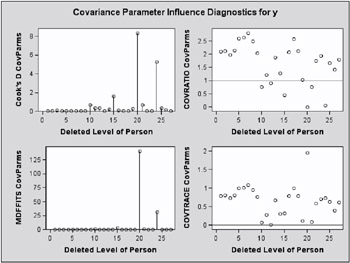
| |
The child who exerts the greatest influence on the fixed effects is subject 24. Maybe surprisingly, this subject impacts the variance-covariance matrix of the fixed effects more than subject 20 (small COVRATIO in Output 46.8.3).
The final model investigated for these data is a random coefficient model as in Stram and Lee (1994) with random effects for the intercept and age effect. The following statements examine the estimates for fixed effects and the entries of the unstructured 2 — 2 variance matrix of the random coefficients graphically.
ods html; ods graphics on; proc mixed data=pr method=ml; class person gender; model y = gender age gender*age / influence(iter=5 effect=person est); random intercept age / type=un subject=person; ods select InfluenceEstParmPanel1 InfluenceEstCovPPanel1; run; ods graphics off; ods html close;
In Output 46.8.4 the graphs on the left-hand side of the panel represent the intercept and slope estimate for boys; the graphs on the right-hand side represent the difference in intercept and slope between boys and girls. Removing any one of the first eleven children, who are girls, does not alter the intercept or slope in the group of boys. The difference in these parameters between boys and girls is altered by the removal of any child. Subject 24 changes the fixed effects considerably, subject 20 much less so. This is consistent with findings based on the unstructured variance-covariance model (Output 46.8.2).
| |
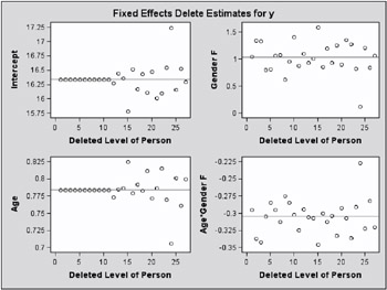
| |
The covariance parameter estimates in Output 46.8.5 show several important features.
-
The panels do not contain information on subject 24. Estimation of the G matrix following removal of that child did not yield a positive definite matrix. As a consequence, covariance parameter diagnostics are not produced for this subject.
-
Subject 20 has great impact on the four covariance parameters. Removing this child from the analysis increases the variance of the random intercept and random slope and reduces the residual variance by almost 80%. The repeated measurements of this child exhibit an up-and-down behavior.
-
The variance of the random intercept and slope are reduced when child 15 is removed from the analysis. This child s growth measurements oscillate about 27.0 from age 10 on.
| |
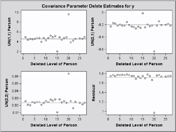
| |
Examining observed and residual values by levels of classification variables is also a useful tool to diagnose the adequacy of the model and unusual observations. Box plots for effects in the model that comprise a single classification variable are requested with the experimental ODS GRAPHICS statement and the experimental BOXPLOT option of the PROC MIXED statement. Since this includes SUBJECT= and GROUP= effects, the statements
ods html; ods graphics on; proc mixed data=pr method=ml boxplot; class person gender; model y = gender age gender*age; random intercept age / type=un subject=person; run; ods graphics off; ods html close;
produce six box plots in the following order: Y by Gender , residual by Gender , Y by Person , residual by Person , and conditional residuals by Gender and Person . The plots for the Person effect are shown in Output 46.8.6 “Output 46.8.8.
Box plots of the observed values show the variation within and between children clearly. The group of girls (subjects 1 “11) is distinguishable from the group of boys by somewhat lesser average growth and lesser within-child variation (Output 46.8.6). After adjusting for overall (population-averaged) gender and age effects, the residual within-child variation is reduced but substantial differences in the means remain (Output 46.8.7). If child-specific inferences are desired, a model accounting for only Gender , Age ,and Gender*Age effects is not adequate for these data.
| |
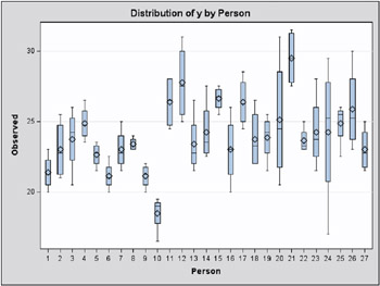
| |
| |
| |
The conditional residuals incorporate the EBLUPs for each child and enable you to examine whether the subject-specific model is adequate (Output 46.8.8). By using each child as its own control the residuals are now centered near zero. Subjects 20 and 24 stand out as unusual in all three sets of box plots.
| |
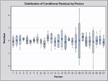
| |
Example 46.9. Examining Individual Test Components
The LCOMPONENTS option of the MODEL statement enables you to perform single degree of freedom tests for individual rows of the L matrix. Such tests are useful to identify interaction patterns. In a balanced layout, Type 3 components of L associated with A * B interactions correspond to simple contrasts of cell mean differences.
The first example revisits the data from the split-plot design by Stroup (1989a) that was analyzed in Example 46.1 on page 2777. Recall that variables A and B represent the whole-plot and subplot factors, respectively.
proc mixed data=sp; class a b block ; modely=aba*b /LComponents e3; random block a*block; run;
The MIXED procedure constructs a separate L matrix for each of the three fixed effects components. The matrices are displayed in Output 46.9.1. The test for fixed effects are shown in Output 46.9.2.
| |
The Mixed Procedure Type 3 Coefficients for A Effect A B Row1 Row2 Intercept A 1 1 A 2 1 A 3 -1 -1 B 1 B 2 A*B 1 1 0.5 A*B 1 2 0.5 A*B 2 1 0.5 A*B 2 2 0.5 A*B 3 1 -0.5 -0.5 A*B 3 2 -0.5 -0.5 Type 3 Coefficients for B Effect A B Row1 Intercept A 1 A 2 A 3 B 1 1 B 2 -1 A*B 1 1 0.3333 A*B 1 2 -0.333 A*B 2 1 0.3333 A*B 2 2 -0.333 A*B 3 1 0.3333 A*B 3 2 -0.333 Type 3 Coefficients for A*B Effect A B Row1 Row2 Intercept A 1 A 2 A 3 B 1 B 2 A*B 1 1 1 A*B 1 2 -1 A*B 2 1 1 A*B 2 2 -1 A*B 3 1 -1 -1 A*B 3 2 1 1
| |
| |
The Mixed Procedure Type 3 Tests of Fixed Effects Num Den Effect DF DF F Value Pr > F A 2 6 4.07 0.0764 B 1 9 19.39 0.0017 A*B 2 9 4.02 0.0566
| |
If ¼ i. denotes a whole-plot main effect mean, ¼ .j denotes a subplot main effect mean, and ¼ ij denotes a cell mean, the five components shown in Output 46.9.3 correspond to tests of
-
H : ¼ 1 . = ¼ 2 .
-
H : ¼ 2 . = ¼ 3 .
-
H : ¼ . 1 = ¼ . 2
-
H : ¼ 11 ˆ’ ¼ 12 = ¼ 31 ˆ’ ¼ 32
-
H : ¼ 21 ˆ’ ¼ 22 = ¼ 31 ˆ’ ¼ 32
| |
The Mixed Procedure L Components of Type 3 Tests of Fixed Effects L Standard Effect Index Estimate Error DF t Value Pr > t A 1 7.1250 3.1672 6 2.25 0.0655 A 2 8.3750 3.1672 6 2.64 0.0383 B 1 5.5000 1.2491 9 4.40 0.0017 A*B 1 7.7500 3.0596 9 2.53 0.0321 A*B 2 7.2500 3.0596 9 2.37 0.0419
| |
The first three components are comparisons of marginal means. The fourth component compares the effect of factor B at the first whole-plot level against the effect of B at the third whole-plot level. Finally, the last component tests whether the factor B effect changes between the second and third whole-plot level.
The Type 3 component tests can also be produced with corresponding ESTIMATE statements.
proc mixed data=sp; class a b block ; model y = a b a*b; random block a*block; estimate a 1 a 1 0 -1; estimate a 2 a 0 1 -1; estimate b 1 b 1 -1; estimate a*b 1 a*b 1 -1 0 0 -1 1; estimate a*b 2 a*b 0 0 1 -1 -1 1; ods select estimates; run;
The Mixed Procedure Estimates Standard Label Estimate Error DF t Value Pr > t a 1 7.1250 3.1672 6 2.25 0.0655 a 2 8.3750 3.1672 6 2.64 0.0383 b 1 5.5000 1.2491 9 4.40 0.0017 a*b 1 7.7500 3.0596 9 2.53 0.0321 a*b 2 7.2500 3.0596 9 2.37 0.0419
A second useful application of the LCOMPONENT option is in polynomial models where Type 1 tests are often used to test the entry of model terms sequentially. The SOLUTION option of the MODEL statement displays the regression coefficients that correspond to a Type 3 analysis, that is,
-
the coefficients represent the partial coefficients you would get by adding the regressor variable last in a model containing all other effects
-
the tests are identical to those in the Type 3 Tests of Fixed Effects table
Consider the following data set and the fit of a third order polynomial regression model.
data polynomial; do x=1 to 20; input y@@; output; end; datalines; 1.092 1.758 1.997 3.154 3.880 3.810 4.921 4.573 6.029 6.032 6.291 7.151 7.154 6.469 7.137 6.374 5.860 4.866 4.155 2.711 ; proc mixed data=polynomial; model y = x x*x x*x*x / s lcomponents htype=1; run;
The t -tests displayed in the Solution for Fixed Effects table are Type 3 tests, sometimes referred to as partial tests. They measure the contribution of a regressor in the presence of all other regressor variables in the model.
The Mixed Procedure Solution for Fixed Effects Standard Effect Estimate Error DF t Value Pr > t Intercept 0.7837 0.3545 16 2.21 0.0420 x 0.3726 0.1426 16 2.61 0.0189 x*x 0.04756 0.01558 16 3.05 0.0076 x*x*x -0.00306 0.000489 16 -6.27 <.0001
The Type 3 L components are identical to the tests in the Solutions for Fixed Effects table. The Type 1 table yields
-
sequential (Type 1) tests of regression variables which test the significance of a regressor given all other variables preceding it in the model list
-
the regression coefficients for sequential submodels
The Mixed Procedure L Components of Type 1 Tests of Fixed Effects L Standard Effect Index Estimate Error DF t Value Pr > t x 1 0.1763 0.01259 16 14.01 <.0001 x*x 1 -0.04886 0.002449 16 -19.95 <.0001 x*x*x 1 -0.00306 0.000489 16 -6.27 <.0001 L Components of Type 3 Tests of Fixed Effects L Standard Effect Index Estimate Error DF t Value Pr > t x 1 0.3726 0.1426 16 2.61 0.0189 x*x 1 0.04756 0.01558 16 3.05 0.0076 x*x*x 1 -0.00306 0.000489 16 -6.27 <.0001
The estimate of 0 . 1763 is the regression coefficient in a simple linear regression of Y on X . The estimate of ˆ’ . 04886 is the partial coefficient for the quadratic term when it is added to a model containing only a linear component. Similarly, the value ˆ’ . 00306 is the partial coefficient for the cubic term when it is added to a model containing a linear and quadratic component. The last Type 1 component is always identical to the corresponding Type 3 component.