Details

Input Data Set

The FACTOR procedure can read an ordinary SAS data set containing raw data or a special data set specified as a TYPE=CORR, TYPE=UCORR, TYPE=SSCP, TYPE=COV, TYPE=UCOV, or TYPE=FACTOR data set containing previously computed statistics. A TYPE=CORR data set can be created by the CORR procedure or various other procedures such as the PRINCOMP procedure. It contains means, standard deviations, the sample size , the correlation matrix, and possibly other statistics if it is created by some procedure other than PROC CORR. A TYPE=COV data set is similar to a TYPE=CORR data set but contains a covariance matrix. A TYPE=UCORR or TYPE=UCOV data set contains a correlation or covariance matrix that is not corrected for the mean. The default VAR variable list does not include Intercept if the DATA= data set is TYPE=SSCP. If the Intercept variable is explicitly specified in the VAR statement with a TYPE=SSCP data set, the NOINT option is activated. A TYPE=FACTOR data set can be created by the FACTOR procedure and is described in the section Output Data Sets on page 1325.

If your data set has many observations and you plan to run FACTOR several times, you can save computer time by first creating a TYPE=CORR data set and using it as input to PROC FACTOR.

  proc corr data=raw out=correl;     /* create TYPE=CORR data set */   proc factor data=correl method=ml; /* maximum likelihood        */   proc factor data=correl;           /* principal components      */  

The data set created by the CORR procedure is automatically given the TYPE=CORR data set option, so you do not have to specify TYPE=CORR. However, if you use a DATA step with a SET statement to modify the correlation data set, you must use the TYPE=CORR attribute in the new data set. You can use a VAR statement with PROC FACTOR when reading a TYPE=CORR data set to select a subset of the variables or change the order of the variables .

Problems can arise from using the CORR procedure when there are missing data. By default, PROC CORR computes each correlation from all observations that have values present for the pair of variables involved (pairwise deletion). The resulting correlation matrix may have negative eigenvalues. If you specify the NOMISS option with the CORR procedure, observations with any missing values are completely omitted from the calculations (listwise deletion), and there is no danger of negative eigenvalues.

PROC FACTOR can also create a TYPE=FACTOR data set, which includes all the information in a TYPE=CORR data set, and use it for repeated analyses. For a TYPE=FACTOR data set, the default value of the METHOD= option is PATTERN. The following statements produce the same PROC FACTOR results as the previous example:

  proc factor data=raw method=ml outstat=fact; /* max. likelihood */   proc factor data=fact method=prin;      /* principal components */  

You can use a TYPE=FACTOR data set to try several different rotation methods on the same data without repeatedly extracting the factors. In the following example, the second and third PROC FACTOR statements use the data set fact created by the first PROC FACTOR statement:

  proc factor data=raw outstat=fact; /* principal components */   proc factor rotate=varimax;        /* varimax rotation     */   proc factor rotate=quartimax;      /* quartimax rotation   */  

You can create a TYPE=CORR, TYPE=UCORR, or TYPE=FACTOR data set in a DATA step. Be sure to specify the TYPE= option in parentheses after the data set name in the DATA statement and include the _TYPE_ and _NAME_ variables. In a TYPE=CORR data set, only the correlation matrix ( _TYPE_ = CORR ) is necessary. It can contain missing values as long as every pair of variables has at least one nonmissing value.

  data correl(type=corr);   _TYPE_='CORR';   input _NAME_$xyz;   datalines;   x  1.0  .   .   y   .7 1.0  .   z   .5  .4 1.0   ;   proc factor;   run;  

You can create a TYPE=FACTOR data set containing only a factor pattern ( _TYPE_ = PATTERN ) and use the FACTOR procedure to rotate it.

  data pat(type=factor);   _TYPE_='PATTERN';   input _NAME_ $ x y z;   datalines;   factor1  .5  .7  .3   factor2  .8  .2  .8   ;   proc factor rotate=promax prerotate=none;   run;  

If the input factors are oblique , you must also include the interfactor correlation matrix with _TYPE_ = FCORR .

  data pat(type=factor);   input _TYPE_ $ _NAME_ $ x y z;   datalines;   pattern factor1  .5  .7  .3   pattern factor2  .8  .2  .8   fcorr   factor1 1.0  .2  .   fcorr   factor2  .2 1.0  .   ;   proc factor rotate=promax prerotate=none;   run;  

Some procedures, such as the PRINCOMP and CANDISC procedures, produce TYPE=CORR or TYPE=UCORR data sets containing scoring coefficients ( _TYPE_ = SCORE or _TYPE_ = USCORE ). These coefficients can be input to PROC FACTOR and rotated by using the METHOD=SCORE option. The input data set must contain the correlation matrix as well as the scoring coefficients.

  proc princomp data=raw n=2 outstat=prin;   run;   proc factor data=prin method=score rotate=varimax;   run;  

Output Data Sets

The OUT= Data Set

The OUT= data set contains all the data in the DATA= data set plus new variables called Factor1 , Factor2 , and so on, containing estimated factor scores. Each estimated factor score is computed as a linear combination of the standardized values of the variables that are factored . The coefficients are always displayed if the OUT= option is specified and they are labeled Standardized Scoring Coefficients.

The OUTSTAT= Data Set

The OUTSTAT= data set is similar to the TYPE=CORR or TYPE=UCORR data set produced by the CORR procedure, but it is a TYPE=FACTOR data set and it contains many results in addition to those produced by PROC CORR. The OUTSTAT= data set contains observations with _TYPE_ = UCORR and _TYPE_ = USTD if you specify the NOINT option.

The output data set contains the following variables:

• the BY variables, if any

• two new character variables, _TYPE_ and _NAME_

• the variables analyzed , that is, those in the VAR statement, or, if there is no VAR statement, all numeric variables not listed in any other statement.

Each observation in the output data set contains some type of statistic as indicated by the _TYPE_ variable. The _NAME_ variable is blank except where otherwise indicated. The values of the _TYPE_ variable are as follows :

_TYPE_	Contents
MEAN	means
STD	standard deviations
USTD	uncorrected standard deviations
N	sample size
CORR	correlations . The _NAME_ variable contains the name of the variable corresponding to each row of the correlation matrix.
UCORR	uncorrected correlations. The _NAME_ variable contains the name of the variable corresponding to each row of the uncorrected correlation matrix.
IMAGE	image coefficients. The _NAME_ variable contains the name of the variable corresponding to each row of the image coefficient matrix.
IMAGECOV	image covariance matrix. The _NAME_ variable contains the name of the variable corresponding to each row of the image covariance matrix.
COMMUNAL	final communality estimates
PRIORS	prior communality estimates, or estimates from the last iteration for iterative methods
WEIGHT	variable weights
SUMWGT	sum of the variable weights
EIGENVAL	eigenvalues
UNROTATE	unrotated factor pattern. The _NAME_ variable contains the name of the factor.
SE_UNROT	standard error estimates for the unrotated loadings. The _NAME_ variable contains the name of the factor.
RESIDUAL	residual correlations. The _NAME_ variable contains the name of the variable corresponding to each row of the residual correlation matrix.
PRETRANS	transformation matrix from prerotation. The _NAME_ variable contains the name of the factor.
PREFCORR	pre-rotated interfactor correlations. The _NAME_ variable contains the name of the factor.
SE_PREFC	standard error estimates for pre-rotated interfactor correlations. The _NAME_ variable contains the name of the factor.
PREROTAT	pre-rotated factor pattern. The _NAME_ variable contains the name of the factor.
SE_PREPA	standard error estimates for the pre-rotated loadings. The _NAME_ variable contains the name of the factor.
PRERCORR	pre-rotated reference axis correlations. The _NAME_ variable contains the name of the factor.
PREREFER	pre-rotated reference structure. The _NAME_ variable contains the name of the factor.
PRESTRUC	pre-rotated factor structure. The _NAME_ variable contains the name of the factor.
SE_PREST	standard error estimates for pre-rotated structure loadings. The _NAME_ variable contains the name of the factor.
PRESCORE	pre-rotated scoring coefficients. The _NAME_ variable contains the name of the factor.
TRANSFOR	transformation matrix from rotation. The _NAME_ variable contains the name of the factor.
FCORR	interfactor correlations. The _NAME_ variable contains the name of the factor.
SE_FCORR	standard error estimates for interfactor correlations. The _NAME_ variable contains the name of the factor.
PATTERN	factor pattern. The _NAME_ variable contains the name of the factor.
SE_PAT	standard error estimates for the rotated loadings. The _NAME_ variable contains the name of the factor.
RCORR	reference axis correlations. The _NAME_ variable contains the name of the factor.
REFERENC	reference structure. The _NAME_ variable contains the name of the factor.
STRUCTUR	factor structure. The _NAME_ variable contains the name of the factor.
SE_STRUC	standard error estimates for structure loadings. The _NAME_ variable contains the name of the factor.
SCORE	scoring coefficients to be applied to standardized variables. The _NAME_ variable contains the name of the factor.
USCORE	scoring coefficients to be applied without subtracting the mean from the raw variables. The _NAME_ variable contains the name of the factor.

Confidence Intervals and the Salience of Factor Loadings

The traditional approach to determining salient loadings (loadings that are considered large in absolute values) employs rules-of-thumb such as 0.3 or 0.4. However, this does not utilize the statistical evidence efficiently . The asymptotic normality of the distribution of factor loadings enables you to construct confidence intervals to gauge the salience of factor loadings. To guarantee the range-respecting properties of confidence intervals, a transformation procedure such as in CEFA (Browne, Cudeck, Tateneni, and Mels 1998) is used. For example, because the orthogonal rotated factor loading must be bounded between ˆ’ 1 and +1, the Fisher transformation

is employed so that is an unbounded parameter. Assuming the asymptotic normality of , a symmetric confidence interval for is constructed . Then, a back-transformation on the confidence limits yields an asymmetric confidence interval for . Applying the results of Browne (1982), a (1 ˆ’ ± )100% confidence interval for the orthogonal factor loading is

where

and is the estimated factor loading, is the standard error estimate of the factor loading, and z _{± / 2} is the (1 ˆ’ ± / 2)100 percentile point of a standard normal distribution.

Once the confidence limits are constructed, you can use the corresponding coverage displays for determining the salience of the variable-factor relationship. In a coverage display, the COVER= value is represented by an asterisk ˜* . The following table summarizes the various displays and their interpretations:

Table 27.2: Interpretations of the Coverage Displays

Positive Estimate	Negative Estimate	COVER=0 specified	Interpretation
[0]*	*[0]		The estimate is not significantly different from zero and the CI covers a region of values that are smaller in magnitude than the COVER= value. This is strong statistical evidence for the non-salience of the variable-factor relationship.
0[ ]*	*[ ]0		The estimate is significantly different from zero but the CI covers a region of values that are smaller in magnitude than the COVER= value. This is strong statistical evidence for the non-salience of the variable-factor relationship.
[0*]	[*0]	[0]	The estimate is not significantly different from zero or the COVER= value. The population value might have been larger or smaller in magnitude than the COVER= value. There is no statistical evidence for the salience of the variable-factor relationship.
0[*]	[*]0		The estimate is significantly different from zero but not from the COVER= value. This is marginal statistical evidence for the salience of the variable-factor relationship.
0*[ ]	[ ]*0	0[ ] or [ ]0	The estimate is significantly different from zero and the CI covers a region of values that are larger in magnitude than the COVER= value. This is strong statistical evidence for the salience of the variable-factor relationship.

See Example 27.4 on page 1369 for an illustration of the use of confidence intervals for interpreting factors.

Simplicity Functions for Rotations

To rotate a factor pattern is to apply a non-singular linear transformation to the unrotated factor pattern matrix. To arrive at an optimal transformation you must define a so-called simplicity function for assessing the optimal point. For the promax or the Procrustean transformation, the simplicity function is defined as the sum of squared differences between the rotated factor pattern and the target matrix. Thus, the solution of the optimal transformation is easily obtained by the familiar least-squares method.

For the class of the generalized Crawford-Ferguson family (Jennrich 1973), the simplicity function being optimized is

where

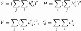
k ₁ , k ₂ , k ₃ , and k ₄ are constants, and b _ij represents an element of the rotated pattern matrix. Except for specialized research purposes, it is rare in practice to use this simplicity function for rotation. However, it reduces to many well-known classes and special cases of rotations. One of these is the Crawford-Ferguson family (Crawford and Ferguson 1970), which minimizes

where c ₁ and c ₂ are constants and ( H ˆ’ Q ) represents variable (row) parsimony and ( V ˆ’ Q ) represents factor (column) parsimony. Therefore, the relative importance of both the variable parsimony and of the factor parsimony is adjusted using the constants c ₁ and c ₂ . The orthomax class (Carroll, see Harman 1976) maximizes the function

where ³ is the orthomax weight and is usually between 0 and the number of variables p . The oblimin class minimizes the function

where is the oblimin weight. For practical purposes, a negative or zero value for is recommended.

All the above definitions are for rotations without row normalization. For rotations with Kaiser normalization the definition of b _ij is replaced by b _ij /h _i , where h _i is the communality of variable i .

Missing Values

If the DATA= data set contains data (rather than a matrix or factor pattern), then observations with missing values for any variables in the analysis are omitted from the computations . If a correlation or covariance matrix is read, it can contain missing values as long as every pair of variables has at least one nonmissing entry. Missing values in a pattern or scoring coefficient matrix are treated as zeros.

Cautions

• The amount of time that FACTOR takes is roughly proportional to the cube of the number of variables. Factoring 100 variables, therefore, takes about 1,000 times as long as factoring 10 variables. Iterative methods (PRINIT, ALPHA, ULS, ML) can also take 100 times as long as noniterative methods (PRINCIPAL, IMAGE, HARRIS).

• No computer program is capable of reliably determining the optimal number of factors since the decision is ultimately subjective . You should not blindly accept the number of factors obtained by default; instead, use your own judgment to make a decision.

• Singular correlation matrices cause problems with the options PRIORS=SMC and METHOD=ML. Singularities can result from using a variable that is the sum of other variables, coding too many dummy variables from a classification variable, or having more variables than observations.

• If you use the CORR procedure to compute the correlation matrix and there are missing data and the NOMISS option is not specified, then the correlation matrix may have negative eigenvalues.

• If a TYPE=CORR, TYPE=UCORR, or TYPE=FACTOR data set is copied or modified using a DATA step, the new data set does not automatically have the same TYPE as the old data set. You must specify the TYPE= data set option in the DATA statement. If you try to analyze a data set that has lost its TYPE=CORR attribute, PROC FACTOR displays a warning message saying that the data set contains _NAME_ and _TYPE_ variables but analyzes the data set as an ordinary SAS data set.

• For a TYPE=FACTOR data set, the default is METHOD=PATTERN, not METHOD=PRIN.

Factor Scores

The FACTOR procedure can compute estimated factor scores directly if you specify the NFACTORS= and OUT= options, or indirectly using the SCORE procedure. The latter method is preferable if you use the FACTOR procedure interactively to determine the number of factors, the rotation method, or various other aspects of the analysis. To compute factor scores for each observation using the SCORE procedure,

• use the SCORE option in the PROC FACTOR statement

• create a TYPE=FACTOR output data set with the OUTSTAT= option

• use the SCORE procedure with both the raw data and the TYPE=FACTOR data set

• do not use the TYPE= option in the PROC SCORE statement

For example, the following statements could be used:

  proc factor data=raw score outstat=fact;   run;   proc score data=raw score=fact out=scores;   run;  

or

  proc corr   data=raw out=correl;   run;   proc factor data=correl score outstat=fact;   run;   proc score  data=raw score=fact out=scores;   run;  

A component analysis (principal, image, or Harris) produces scores with mean zero and variance one. If you have done a common factor analysis, the true factor scores have mean zero and variance one, but the computed factor scores are only estimates of the true factor scores. These estimates have mean zero but variance equal to the squared multiple correlation of the factor with the variables. The estimated factor scores may have small nonzero correlations even if the true factors are uncorrelated.

Variable Weights and Variance Explained

A principal component analysis of a correlation matrix treats all variables as equally important. A principal component analysis of a covariance matrix gives more weight to variables with larger variances. A principal component analysis of a covariance matrix is equivalent to an analysis of a weighted correlation matrix, where the weight of each variable is equal to its variance. Variables with large weights tend to have larger loadings on the first component and smaller residual correlations than variables with small weights.

You may want to give weights to variables using values other than their variances. Mulaik (1972) explains how to obtain a maximally reliable component by means of a weighted principal component analysis. With the FACTOR procedure, you can indirectly give arbitrary weights to the variables by using the COV option and rescaling the variables to have variance equal to the desired weight, or you can give arbitrary weights directly by using the WEIGHT option and including the weights in a TYPE=CORR data set.

Arbitrary variable weights can be used with the METHOD=PRINCIPAL, METHOD=PRINIT, METHOD=ULS, or METHOD=IMAGE option. Alpha and ML factor analyses compute variable weights based on the communalities (Harman 1976, pp. 217-218). For alpha factor analysis, the weight of a variable is the reciprocal of its communality. In ML factor analysis, the weight is the reciprocal of the uniqueness. Harris component analysis uses weights equal to the reciprocal of one minus the squared multiple correlation of each variable with the other variables.

For uncorrelated factors, the variance explained by a factor can be computed with or without taking the weights into account. The usual method for computing variance accounted for by a factor is to take the sum of squares of the corresponding column of the factor pattern, yielding an unweighted result. If the square of each loading is multiplied by the weight of the variable before the sum is taken, the result is the weighted variance explained, which is equal to the corresponding eigenvalue except in image analysis. Whether the weighted or unweighted result is more important depends on the purpose of the analysis.

In the case of correlated factors, the variance explained by a factor can be computed with or without taking the other factors into account. If you want to ignore the other factors, the variance explained is given by the weighted or unweighted sum of squares of the appropriate column of the factor structure since the factor structure contains simple correlations. If you want to subtract the variance explained by the other factors from the amount explained by the factor in question (the Type II variance explained), you can take the weighted or unweighted sum of squares of the appropriate column of the reference structure because the reference structure contains semipartial correlations. There are other ways of measuring the variance explained. For example, given a prior ordering of the factors, you can eliminate from each factor the variance explained by previous factors and compute a Type I variance explained. Harman (1976, pp. 268-270) provides another method, which is based on direct and joint contributions.

Heywood Cases and Other Anomalies

Since communalities are squared correlations, you would expect them always to lie between 0 and 1. It is a mathematical peculiarity of the common factor model, however, that final communality estimates may exceed 1. If a communality equals 1, the situation is referred to as a Heywood case, and if a communality exceeds 1, it is an ultra-Heywood case. An ultra -Heywood case implies that some unique factor has negative variance, a clear indication that something is wrong. Possible causes include

• bad prior communality estimates

• too many common factors

• too few common factors

• not enough data to provide stable estimates

• the common factor model is not an appropriate model for the data

An ultra-Heywood case renders a factor solution invalid. Factor analysts disagree about whether or not a factor solution with a Heywood case can be considered legitimate .

Theoretically, the communality of a variable should not exceed its reliability. Violation of this condition is called a quasi-Heywood case and should be regarded with the same suspicion as an ultra-Heywood case.

Elements of the factor structure and reference structure matrices can exceed 1 only in the presence of an ultra-Heywood case. On the other hand, an element of the factor pattern may exceed 1 in an oblique rotation.

The maximum likelihood method is especially susceptible to quasi- or ultra-Heywood cases. During the iteration process, a variable with high communality is given a high weight; this tends to increase its communality, which increases its weight, and so on.

It is often stated that the squared multiple correlation of a variable with the other variables is a lower bound to its communality. This is true if the common factor model fits the data perfectly , but it is not generally the case with real data. A final communality estimate that is less than the squared multiple correlation can, therefore, indicate poor fit, possibly due to not enough factors. It is by no means as serious a problem as an ultra-Heywood case. Factor methods using the Newton-Raphson method can actually produce communalities less than 0, a result even more disastrous than an ultra-Heywood case.

The squared multiple correlation of a factor with the variables may exceed 1, even in the absence of ultra-Heywood cases. This situation is also cause for alarm. Alpha factor analysis seems to be especially prone to this problem, but it does not occur with maximum likelihood. If a squared multiple correlation is negative, there are too many factors retained.

With data that do not fit the common factor model perfectly, you can expect some of the eigenvalues to be negative. If an iterative factor method converges properly, the sum of the eigenvalues corresponding to rejected factors should be 0; hence, some eigenvalues are positive and some negative. If a principal factor analysis fails to yield any negative eigenvalues, the prior communality estimates are probably too large. Negative eigenvalues cause the cumulative proportion of variance explained to exceed 1 for a sufficiently large number of factors. The cumulative proportion of variance explained by the retained factors should be approximately 1 for principal factor analysis and should converge to 1 for iterative methods. Occasionally, a single factor can explain more than 100 percent of the common variance in a principal factor analysis, indicating that the prior communality estimates are too low.

If a squared canonical correlation or a coefficient alpha is negative, there are too many factors retained.

Principal component analysis, unlike common factor analysis, has none of these problems if the covariance or correlation matrix is computed correctly from a data set with no missing values. Various methods for missing value correlation or severe rounding of the correlations can produce negative eigenvalues in principal components.

Time Requirements

n	=	number of observations
v	=	number of variables
f	=	number of factors
i	=	number of iterations during factor extraction
r	=	length of iterations during factor rotation

The time required to compute	is roughly proportional to
an overall factor analysis	iv 3
the correlation matrix	nv 2
PRIORS=SMC or ASMC	v 3
PRIORS=MAX	v 2
eigenvalues	v 3
final eigenvectors	fv 2
generalized Crawford-Ferguson family of rotations, PROMAX, or HK	rvf 2
ROTATE=PROCRUSTES	vf 2

Each iteration in the PRINIT or ALPHA method requires computation of eigenvalues and f eigenvectors.

Each iteration in the ML or ULS method requires computation of eigenvalues and v ˆ’ f eigenvectors.

The amount of time that PROC FACTOR takes is roughly proportional to the cube of the number of variables. Factoring 100 variables, therefore, takes about 1000 times as long as factoring 10 variables. Iterative methods (PRINIT, ALPHA, ULS, ML) can also take 100 times as long as noniterative methods (PRINCIPAL, IMAGE, HARRIS).

Displayed Output

PROC FACTOR output includes

• Mean and Std Dev (standard deviation) of each variable and the number of observations, if you specify the SIMPLE option

• Correlations, if you specify the CORR option

• Inverse Correlation Matrix, if you specify the ALL option

• Partial Correlations Controlling all other Variables (negative anti-image correlations), if you specify the MSA option. If the data are appropriate for the common factor model, the partial correlations should be small.

• Kaiser s Measure of Sampling Adequacy (Kaiser 1970; Kaiser and Rice 1974; Cerny and Kaiser 1977) both overall and for each variable, if you specify the MSA option. The MSA is a summary of how small the partial correlations are relative to the ordinary correlations. Values greater than 0.8 can be considered good. Values less than 0.5 require remedial action, either by deleting the offending variables or by including other variables related to the offenders.

• Prior Communality Estimates, unless 1.0s are used or unless you specify the METHOD=IMAGE, METHOD=HARRIS, METHOD=PATTERN, or METHOD=SCORE option

• Squared Multiple Correlations of each variable with all the other variables, if you specify the METHOD=IMAGE or METHOD=HARRIS option

• Image Coefficients, if you specify the METHOD=IMAGE option

• Image Covariance Matrix, if you specify the METHOD=IMAGE option

• Preliminary Eigenvalues based on the prior communalities, if you specify the METHOD=PRINIT, METHOD=ALPHA, METHOD=ML, or METHOD=ULS option. The table produced includes the Total and the Average of the eigenvalues, the Difference between successive eigenvalues, the Proportion of variation represented, and the Cumulative proportion of variation.

• the number of factors that are retained, unless you specify the METHOD=PATTERN or METHOD=SCORE option

• the Scree Plot of Eigenvalues, if you specify the SCREE option. The preliminary eigenvalues are used if you specify the METHOD=PRINIT, METHOD=ALPHA, METHOD=ML, or METHOD=ULS option.

• the iteration history, if you specify the METHOD=PRINIT, METHOD=ALPHA, METHOD=ML, or METHOD=ULS option. The table produced contains the iteration number (Iter); the Criterion being optimized (J reskog 1977); the Ridge value for the iteration if you specify the METHOD=ML or METHOD=ULS option; the maximum Change in any communality estimate; and the Communalities.

• Significance tests, if you specify the option METHOD=ML, including Bartlett s Chi-square, df, and Prob > ² for H : No common factors and H : factors retained are sufficient to explain the correlations. The variables should have an approximate multivariate normal distribution for the probability levels to be valid. Lawley and Maxwell (1971) suggest that the number of observations should exceed the number of variables by fifty or more, although Geweke and Singleton (1980) claim that as few as ten observations are adequate with five variables and one common factor. Certain regularity conditions must also be satisfied for Bartlett s ² test to be valid (Geweke and Singleton 1980), but in practice these conditions usually are satisfied. The notation Prob>chi**2 means the probability under the null hypothesis of obtaining a greater ² statistic than that observed . The Chi-square value is displayed with and without Bartlett s correction.

• Akaike s Information Criterion, if you specify the METHOD=ML option. Akaike s information criterion (AIC) (Akaike 1973, 1974, 1987) is a general criterion for estimating the best number of parameters to include in a model when maximum likelihood estimation is used. The number of factors that yields the smallest value of AIC is considered best. Like the chi-square test, AIC tends to include factors that are statistically significant but inconsequential for practical purposes.

• Schwarz s Bayesian Criterion, if you specify the METHOD=ML option. Schwarz s Bayesian Criterion (SBC) (Schwarz 1978) is another criterion, similar to AIC, for determining the best number of parameters. The number of factors that yields the smallest value of SBC is considered best; SBC seems to be less inclined to include trivial factors than either AIC or the chi-square test.

• Tucker and Lewis s Reliability Coefficient, if you specify the METHOD=ML option (Tucker and Lewis 1973)

• Squared Canonical Correlations, if you specify the METHOD=ML option. These are the same as the squared multiple correlations for predicting each factor from the variables.

• Coefficient Alpha for Each Factor, if you specify the METHOD=ALPHA option

• Eigenvectors, if you specify the EIGENVECTORS or ALL option, unless you also specify the METHOD=PATTERN or METHOD=SCORE option

• Eigenvalues of the (Weighted) (Reduced) (Image) Correlation or Covariance Matrix, unless you specify the METHOD=PATTERN or METHOD=SCORE option. Included are the Total and the Average of the eigenvalues, the Difference between successive eigenvalues, the Proportion of variation represented, and the Cumulative proportion of variation.

• the Factor Pattern, which is equal to both the matrix of standardized regression coefficients for predicting variables from common factors and the matrix of correlations between variables and common factors since the extracted factors are uncorrelated. Standard error estimates are included if the SE option is specified with METHOD=ML. Confidence limits and coverage displays are included if COVER= option is specified with METHOD=ML.

• Variance explained by each factor, both Weighted and Unweighted, if variable weights are used

• Final Communality Estimates, including the Total communality; or Final Communality Estimates and Variable Weights, including the Total communality, both Weighted and Unweighted, if variable weights are used. Final communality estimates are the squared multiple correlations for predicting the variables from the estimated factors, and they can be obtained by taking the sum of squares of each row of the factor pattern, or a weighted sum of squares if variable weights are used.

• Residual Correlations with Uniqueness on the Diagonal, if you specify the RESIDUAL or ALL option

• Root Mean Square Off-diagonal Residuals, both Over-all and for each variable, if you specify the RESIDUAL or ALL option

• Partial Correlations Controlling Factors, if you specify the RESIDUAL or ALL option

• Root Mean Square Off-diagonal Partials , both Over-all and for each variable, if you specify the RESIDUAL or ALL option

• Plots of Factor Pattern for unrotated factors, if you specify the PREPLOT option. The number of plots is determined by the NPLOT= option.

• Variable Weights for Rotation, if you specify the NORM=WEIGHT option

• Factor Weights for Rotation, if you specify the HKPOWER= option

• Orthogonal Transformation Matrix, if you request an orthogonal rotation

• Rotated Factor Pattern, if you request an orthogonal rotation. Standard error estimates are included if the SE option is specified with METHOD=ML. Confidence limits and coverage displays are included if COVER= option is specified with METHOD=ML.

• Variance explained by each factor after rotation. If you request an orthogonal rotation and if variable weights are used, both weighted and unweighted values are produced.

• Target Matrix for Procrustean Transformation, if you specify the ROTATE=PROMAX or ROTATE=PROCRUSTES option

• the Procrustean Transformation Matrix, if you specify the ROTATE=PROMAX or ROTATE=PROCRUSTES option

• the Normalized Oblique Transformation Matrix, if you request an oblique rotation, which, for the option ROTATE=PROMAX, is the product of the prerotation and the Procrustean rotation

• Inter-factor Correlations, if you specify an oblique rotation. Standard error estimates are included if the SE option is specified with METHOD=ML. Confidence limits and coverage displays are included if COVER= option is specified with METHOD=ML.

• Rotated Factor Pattern (Std Reg Coefs), if you specify an oblique rotation, giving standardized regression coefficients for predicting the variables from the factors. Standard error estimates are included if the SE option is specified with METHOD=ML. Confidence limits and coverage displays are included if COVER= option is specified with METHOD=ML.

• Reference Axis Correlations if you specify an oblique rotation. These are the partial correlations between the primary factors when all factors other than the two being correlated are partialed out.

• Reference Structure (Semipartial Correlations), if you request an oblique rotation. The reference structure is the matrix of semipartial correlations (Kerlinger and Pedhazur 1973) between variables and common factors, removing from each common factor the effects of other common factors. If the common factors are uncorrelated, the reference structure is equal to the factor pattern.

• Variance explained by each factor eliminating the effects of all other factors, if you specify an oblique rotation. Both Weighted and Unweighted values are produced if variable weights are used. These variances are equal to the (weighted) sum of the squared elements of the reference structure corresponding to each factor.

• Factor Structure (Correlations), if you request an oblique rotation. The (primary) factor structure is the matrix of correlations between variables and common factors. If the common factors are uncorrelated, the factor structure is equal to the factor pattern. Standard error estimates are included if the SE option is specified with METHOD=ML. Confidence limits and coverage displays are included if COVER= option is specified with METHOD=ML.

• Variance explained by each factor ignoring the effects of all other factors, if you request an oblique rotation. Both Weighted and Unweighted values are produced if variable weights are used. These variances are equal to the (weighted) sum of the squared elements of the factor structure corresponding to each factor.

• Final Communality Estimates for the rotated factors if you specify the ROTATE= option. The estimates should equal the unrotated communalities.

• Squared Multiple Correlations of the Variables with Each Factor, if you specify the SCORE or ALL option, except for unrotated principal components

• Standardized Scoring Coefficients, if you specify the SCORE or ALL option

• Plots of the Factor Pattern for rotated factors, if you specify the PLOT option and you request an orthogonal rotation. The number of plots is determined by the NPLOT= option.

• Plots of the Reference Structure for rotated factors, if you specify the PLOT option and you request an oblique rotation. The number of plots is determined by the NPLOT= option. Included are the Reference Axis Correlation and the Angle between the Reference Axes for each pair of factors plotted.

If you specify the ROTATE=PROMAX option, the output includes results for both the prerotation and the Procrustean rotation.

ODS Table Names

PROC FACTOR assigns a name to each table it creates. You can use these names to reference the table when using the Output Delivery System (ODS) to select tables and create output data sets. These names are listed in the following table. For more information on ODS, see Chapter 14, Using the Output Delivery System.

Table 27.3: ODS Tables Produced in PROC FACTOR

ODS Table Name	Description	Option
AlphaCoef	Coefficient alpha for each factor	METHOD=ALPHA
CanCorr	Squared canonical correlations	METHOD=ML
CondStdDev	Conditional standard deviations	SIMPLE w/PARTIAL
ConvergenceStatus	Convergence status	METHOD=PRINIT, =ALPHA, =ML, or =ULS
Corr	Correlations	CORR
Eigenvalues	Eigenvalues	default, SCREE
Eigenvectors	Eigenvectors	EIGENVECTORS
FactorWeightRotate	Factor weights for rotation	HKPOWER=
FactorPattern	Factor pattern	default
FactorStructure	Factor structure	ROTATE= any oblique rotation
FinalCommun	Final communalities	default
FinalCommunWgt	Final communalities with weights	METHOD=ML, METHOD=ALPHA
FitMeasures	Measures of fit	METHOD=ML
ImageCoef	Image coefficients	METHOD=IMAGE
ImageCov	Image covariance matrix	METHOD=IMAGE
ImageFactors	Image factor matrix	METHOD=IMAGE
InputFactorPattern	Input factor pattern	METHOD=PATTERN with PRINT or ALL
InputScoreCoef	Standardized input scoring coefficients	METHOD=SCORE with PRINT or ALL
InterFactorCorr	Inter-factor correlations	ROTATE= any oblique rotation
InvCorr	Inverse correlation matrix	ALL
IterHistory	Iteration history	METHOD=PRINIT, =ALPHA, =ML, or =ULS
MultipleCorr	Squared multiple correlations	METHOD=IMAGE or METHOD=HARRIS
NormObliqueTrans	Normalized oblique transformation matrix	ROTATE= any oblique rotation
ObliqueRotFactPat	Rotated factor pattern	ROTATE= any oblique rotation
ObliqueTrans	Oblique transformation matrix	HKPOWER=
OrthRotFactPat	Rotated factor pattern	ROTATE= any orthogonal rotation
OrthTrans	Orthogonal transformation matrix	ROTATE= any orthogonal rotation
ParCorrControlFactor	Partial correlations controlling factors	RESIDUAL
ParCorrControlVar	Partial correlations controlling other variables	MSA
PartialCorr	Partial correlations	MSA, CORR w/PARTIAL
PriorCommunalEst	Prior communality estimates	PRIORS=, METHOD=ML, METHOD=ALPHA
ProcrustesTarget	Target matrix for Procrustean transformation	ROTATE=PROCRUSTES, ROTATE=PROMAX
ProcrustesTrans	Procrustean transformation matrix	ROTATE=PROCRUSTES, ROTATE=PROMAX
RMSOffDiagPartials	Root mean square off-diagonal partials	RESIDUAL
RMSOffDiagResids	Root mean square off-diagonal residuals	RESIDUAL
ReferenceAxisCorr	Reference axis correlations	ROTATE= any oblique rotation
ReferenceStructure	Reference structure	ROTATE= any oblique rotation
ResCorrUniqueDiag	Residual correlations with uniqueness on the diagonal	RESIDUAL
SamplingAdequacy	Kaiser s measure of sampling adequacy	MSA
SignifTests	Significance tests	METHOD=ML
SimpleStatistics	Simple statistics	SIMPLE
StdScoreCoef	Standardized scoring coefficients	SCORE
VarExplain	Variance explained	default
VarExplainWgt	Variance explained with weights	METHOD=ML, METHOD=ALPHA
VarFactorCorr	Squared multiple correlations of the variables with each factor	SCORE
VarWeightRotate	Variable weights for rotation	NORM=WEIGHT, ROTATE=