Chapter 2: Introduction to Regression Procedures | SAS/STAT 9.1 Users Guide, Volumes 1-7

Overview

This chapter reviews SAS/STAT software procedures that are used for regression analysis: CATMOD, GLM, LIFEREG, LOESS, LOGISTIC, NLIN, ORTHOREG, PLS, PROBIT, ROBUSTREG, REG, RSREG, and TRANSREG. The REG procedure provides the most general analysis capabilities; the other procedures give more specialized analyses. This chapter also briefly mentions several procedures in SAS/ETS software.

Introduction

Many SAS/STAT procedures, each with special features, perform regression analysis. The following procedures perform at least one type of regression analysis:

CATMOD	analyzes data that can be represented by a contingency table. PROC CATMOD fits linear models to functions of response frequencies, and it can be used for linear and logistic regression. See Chapter 4, Introduction to Categorical Data Analysis Procedures, and Chapter 22, The CATMOD Procedure, for more information.
GENMOD	fits generalized linear models. PROC GENMOD is especially suited for responses with discrete outcomes , and it performs logistic regression and Poisson regression as well as fitting Generalized Estimating Equations for repeated measures data. See Chapter 4, Introduction to Categorical Data Analysis Procedures, and Chapter 31, The GENMOD Procedure, for more information.
GLM	uses the method of least squares to fit general linear models. In addition to many other analyses, PROC GLM can perform simple, multiple, polynomial, and weighted regression. PROC GLM has many of the same input/output capabilities as PROC REG, but it does not provide as many diagnostic tools or allow interactive changes in the model or data. See Chapter 3, Introduction to Analysis-of-Variance Procedures, and Chapter 32, The GLM Procedure, for more information.
LIFEREG	fits parametric models to failure-time data that may be right censored. These types of models are commonly used in survival analysis. See Chapter 9, Introduction to Survival Analysis Procedures, and Chapter 39, The LIFEREG Procedure, for more information.
LOESS	fits nonparametric models using a local regression method. PROC LOESS is suitable for modeling regression surfaces where the underlying parametric form is unknown and where robustness in the presence of ouliers is required. See Chapter 41, The LOESS Procedure, for more information.
LOGISTIC	fits logistic models for binomial and ordinal outcomes. PROC LOGISTIC provides a wide variety of model-building methods and computes numerous regression diagnostics. See Chapter 4, Introduction to Categorical Data Analysis Procedures, and Chapter 42, The LOGISTIC Procedure, for more information.
NLIN	builds nonlinear regression models. Several different iterative methods are available. See Chapter 50, The NLIN Procedure, for more information.
ORTHOREG	performs regression using the Gentleman-Givens computational method. For ill-conditioned data, PROC ORTHOREG can produce more accurate parameter estimates than other procedures such as PROC GLM and PROC REG. See Chapter 53, The ORTHOREG Procedure, for more information.
PLS	performs partial least squares regression, principal components regression, and reduced rank regression, with cross validation for the number of components . See Chapter 56, The PLS Procedure, for more information.
PROBIT	performs probit regression as well as logistic regression and ordinal logistic regression. The PROBIT procedure is useful when the dependent variable is either dichotomous or polychotomous and the independent variables are continuous. See Chapter 60, The PROBIT Procedure, for more information.
REG	performs linear regression with many diagnostic capabilities, selects models using one of nine methods, produces scatter plots of raw data and statistics, highlights scatter plots to identify particular observations, and allows interactive changes in both the regression model and the data used to fit the model. See Chapter 61, The REG Procedure, for more information.
ROBUSTREG	performs robust regression using Huber M estimation and high breakdown value estimation. PROC ROBUSTREG is suitable for detecting outliers and providing resistant (stable) results in the presence of outliers. See Chapter 62, The ROBUSTREG Procedure, for more information.
RSREG	builds quadratic response-surface regression models. PROC RSREG analyzes the fitted response surface to determine the factor levels of optimum response and performs a ridge analysis to search for the region of optimum response. See Chapter 63, The RSREG Procedure, for more information.
TRANSREG	fits univariate and multivariate linear models, optionally with spline and other nonlinear transformations. Models include ordinary regression and ANOVA, multiple and multivariate regression, metric and nonmetric conjoint analysis, metric and nonmetric vector and ideal point preference mapping, redundancy analysis, canonical correlation, and response surface regression. See Chapter 75, The TRANSREG Procedure, for more information.
Several SAS/ETS procedures also perform regression. The following procedures are documented in the SAS/ETS User s Guide .
AUTOREG	implements regression models using time-series data where the errors are autocorrelated. Refer to ?? for more details.
PDLREG	performs regression analysis with polynomial distributed lags. Refer to ?? for more details.
SYSLIN	handles linear simultaneous systems of equations, such as econometric models. Refer to ?? for more details.
MODEL	handles nonlinear simultaneous systems of equations, such as econometric models. Refer to ?? for more details.

Introductory Example

Regression analysis is the analysis of the relationship between one variable and another set of variables. The relationship is expressed as an equation that predicts a response variable (also called a dependent variable or criterion ) from a function of regressor variables (also called independent variables, predictors, explanatory variables, factors, or carriers ) and parameters . The parameters are adjusted so that a measure of fit is optimized. For example, the equation for the i th observation might be

where y _i is the response variable, x _i is a regressor variable, ² and ² ₁ are unknown parameters to be estimated, and ˆˆ _i is an error term .

You might use regression analysis to find out how well you can predict a child s weight if you know that child s height. Suppose you collect your data by measuring heights and weights of 19 school children. You want to estimate the intercept ² and the slope ² ₁ of a line described by the equation

where

Weight	is the response variable.
² , ² ₁	are the unknown parameters.
Height	is the regressor variable.
ˆˆ	is the unknown error.

The data are included in the following program. The results are displayed in Figure 2.1 and Figure 2.2.

  The REG Procedure   Model: MODEL1   Dependent Variable: Weight   Analysis of Variance   Sum of           Mean   Source                   DF        Squares         Square    F Value    Pr > F   Model                     1     7193.24912     7193.24912      57.08    <.0001   Error                    17     2142.48772      126.02869   Corrected Total          18     9335.73684   Root MSE             11.22625    R-Square     0.7705   Dependent Mean      100.02632    Adj R-Sq     0.7570   Coeff Var            11.22330   Parameter Estimates   Parameter       Standard   Variable     DF       Estimate          Error    t Value    Pr > t   Intercept     1   143.02692       32.27459   4.43      0.0004   Height        1        3.89903        0.51609       7.55      <.0001

Figure 2.1: Regression for Weight and Height Data

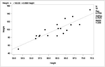
Figure 2.2: Regression for Weight and Height Data

  data class;   input Name $ Height Weight Age;   datalines;   Alfred  69.0 112.5 14   Alice   56.5  84.0 13   Barbara 65.3  98.0 13   Carol   62.8 102.5 14   Henry   63.5 102.5 14   James   57.3  83.0 12   Jane    59.8  84.5 12   Janet   62.5 112.5 15   Jeffrey 62.5  84.0 13   John    59.0  99.5 12   Joyce   51.3  50.5 11   Judy    64.3  90.0 14   Louise  56.3  77.0 12   Mary    66.5 112.0 15   Philip  72.0 150.0 16   Robert  64.8 128.0 12   Ronald  67.0 133.0 15   Thomas  57.5  85.0 11   William 66.5 112.0 15   ;   symbol1 v=dot c=blue height=3.5pct;   proc reg;   model Weight=Height;   plot Weight*Height/cframe=ligr;   run;

Estimates of ² and ² ₁ for these data are b = ˆ’ 143 . 0 and b ₁ = 3 . 9, so the line is described by the equation

Regression is often used in an exploratory fashion to look for empirical relationships, such as the relationship between Height and Weight . In this example, Height is not the cause of Weight . You would need a controlled experiment to confirm scientifically the relationship. See the Comments on Interpreting Regression Statistics section on page 42 for more information.

The method most commonly used to estimate the parameters is to minimize the sum of squares of the differences between the actual response value and the value predicted by the equation. The estimates are called least-squares estimates , and the criterion value is called the error sum of squares

where b and b ₁ are the estimates of ² and ² ₁ that minimize SSE.

For a general discussion of the theory of least-squares estimation of linear models and its application to regression and analysis of variance, refer to one of the applied regression texts , including Draper and Smith (1981), Daniel and Wood (1980), Johnston (1972), and Weisberg (1985).

SAS/STAT regression procedures produce the following information for a typical regression analysis.

parameter estimates using the least-squares criterion
estimates of the variance of the error term
estimates of the variance or standard deviation of the sampling distribution of the parameter estimates
tests of hypotheses about the parameters

SAS/STAT regression procedures can produce many other specialized diagnostic statistics, including

collinearity diagnostics to measure how strongly regressors are related to other regressors and how this affects the stability and variance of the estimates (REG)
influence diagnostics to measure how each individual observation contributes to determining the parameter estimates, the SSE, and the fitted values (LOGISTIC, REG, RSREG)
lack-of-fit diagnostics that measure the lack of fit of the regression model by comparing the error variance estimate to another pure error variance that is not dependent on the form of the model (CATMOD, PROBIT, RSREG)
diagnostic scatter plots that check the fit of the model and highlighted scatter plots that identify particular observations or groups of observations (REG)
predicted and residual values, and confidence intervals for the mean and for an individual value (GLM, LOGISTIC, REG)
time-series diagnostics for equally spaced time-series data that measure how much errors may be related across neighboring observations. These diagnostics can also measure functional goodness of fit for data sorted by regressor or response variables (REG, SAS/ETS procedures).

General Regression: The REG Procedure

The REG procedure is a general-purpose procedure for regression that

handles multiple regression models
provides nine model-selection methods
allows interactive changes both in the model and in the data used to fitthe model
allows linear equality restrictions on parameters
tests linear hypotheses and multivariate hypotheses
produces collinearity diagnostics, influence diagnostics, and partial regression leverage plots
saves estimates, predicted values, residuals, confidence limits, and other diagnostic statistics in output SAS data sets
generates plots of data and of various statistics
paints or highlights scatter plots to identify particular observations or groups of observations
uses, optionally, correlations or crossproducts for input

Model-selection Methods in PROC REG

The nine methods of model selection implemented in PROC REG are

NONE	no selection. This method is the default and uses the full model given in the MODEL statement to fit the linear regression.
FORWARD	forward selection. This method starts with no variables in the model and adds variables one by one to the model. At each step, the variable added is the one that maximizes the fit of the model. You can also specify groups of variables to treat as a unit during the selection process. An option enables you to specify the criterion for inclusion.
BACKWARD	backward elimination . This method starts with a full model and eliminates variables one by one from the model. At each step, the variable with the smallest contribution to the model is deleted. You can also specify groups of variables to treat as a unit during the selection process. An option enables you to specify the criterion for exclusion.
STEPWISE	stepwise regression, forward and backward. This method is a modification of the forward-selection method in that variables already in the model do not necessarily stay there. You can also specify groups of variables to treat as a unit during the selection process. Again, options enable you to specify criteria for entry into the model and for remaining in the model.
MAXR	maximum R ² improvement. This method tries to find the best one-variable model, the best two-variable model, and so on. The MAXR method differs from the STEPWISE method in that many more models are evaluated with MAXR, which considers all switches before making any switch. The STEPWISE method may remove the worst variable without considering what the best remaining variable might accomplish, whereas MAXR would consider what the best remaining variable might accomplish. Consequently, MAXR typically takes much longer to run than STEPWISE.
MINR	minimum R ² improvement. This method closely resembles MAXR, but the switch chosen is the one that produces the smallest increase in R ² .
RSQUARE	finds a specified number of models having the highest R ² in each of a range of model sizes.
CP	finds a specified number of models with the lowest C _p within a range of model sizes.
ADJRSQ	finds a specified number of models having the highest adjusted R ² within a range of model sizes.

Nonlinear Regression: The NLIN Procedure

The NLIN procedure implements iterative methods that attempt to find least-squares estimates for nonlinear models. The default method is Gauss-Newton, although several other methods, such as Newton and Marquardt, are available. You must specify parameter names , starting values, and expressions for the model. All necessary analytical derivatives are calculated automatically for you. Grid search is also available to select starting values for the parameters. Since nonlinear models are often difficult to estimate, PROC NLIN may not always find the globally optimal least-squares estimates.

Response Surface Regression: The RSREG Procedure

The RSREG procedure fits a quadratic response-surface model, which is useful in searching for factor values that optimize a response. The following features in PROC RSREG make it preferable to other regression procedures for analyzing response surfaces:

automatic generation of quadratic effects
a lack-of-fittest
solutions for critical values of the surface
eigenvalues of the associated quadratic form
a ridge analysis to search for the direction of optimum response

Partial Least Squares Regression: The PLS Procedure

The PLS procedure fits models using any one of a number of linear predictive methods, including partial least squares (PLS). Ordinary least-squares regression, as implemented in SAS/STAT procedures such as PROC GLM and PROC REG, has the single goal of minimizing sample response prediction error, seeking linear functions of the predictors that explain as much variation in each response as possible. The techniques implemented in the PLS procedure have the additional goal of accounting for variation in the predictors, under the assumption that directions in the predictor space that are well sampled should provide better prediction for new observations when the predictors are highly correlated. All of the techniques implemented in the PLS procedure work by extracting successive linear combinations of the predictors, called factors (also called components or latent vectors ), which optimally address one or both of these two goals ”explaining response variation and explaining predictor variation. In particular, the method of partial least squares balances the two objectives, seeking for factors that explain both response and predictor variation.

Regression for Ill-conditioned Data: The ORTHOREG Procedure

The ORTHOREG procedure performs linear least-squares regression using the Gentleman-Givens computational method, and it can produce more accurate parameter estimates for ill-conditioned data. PROC GLM and PROC REG produce very accurate estimates for most problems. However, if you have very ill-conditioned data, consider using the ORTHOREG procedure. The collinearity diagnostics in PROC REG can help you to determine whether PROC ORTHOREG would be useful.

Local Regression: The LOESS Procedure

The LOESS procedure implements a nonparametric method for estimating regression surfaces pioneered by Cleveland, Devlin, and Grosse (1988). The LOESS procedure allows great flexibility because no assumptions about the parametric form of the regression surface are needed. Furthermore, the LOESS procedure is suitable when there are outliers in the data and a robust fitting method is necessary.

Robust Regression: The ROBUSTREG Procedure

The ROBUSTREG procedure implements algorithms to detect outliers and provide resistant (stable) results in the presence of outliers. The ROBUSTREG procedure provides four such methods: M estimation, LTS estimation, S estimation, and MM estimation.

M estimation was introduced by Huber (1973), and it is the simplest approach both computationally and theoretically. Although it is not robust with respect to leverage points, it is still used extensively in analyzing data for which it can be assumed that the contamination is mainly in the response direction.
Least Trimmed Squares (LTS) estimation is a high breakdown value method introduced by Rousseeuw (1984). The breakdown value is a measure of the proportion of contamination that an estimation method can withstand and still maintain its robustness.
S estimation is a high breakdown value method introduced by Rousseeuw and Yohai (1984). With the same breakdown value, it has a higher statistical efficiency than LTS estimation.
MM estimation, introduced by Yohai (1987), combines high breakdown value estimation and M estimation. It has both the high breakdown property and a higher statistical efficiency than S estimation.

Logistic Regression: The LOGISTIC Procedure

The LOGISTIC procedure fits logistic models, in which the response can be either dichotomous or polychotomous. Stepwise model selection is available. You can request regression diagnostics, and predicted and residual values.

Regression with Transformations: The TRANSREG Procedure

The TRANSREG procedure can fit many standard linear models. In addition, PROC TRANSREG can find nonlinear transformations of data and fit a linear model to the transformed variables. This is in contrast to PROC REG and PROC GLM, which fit linear models to data, or PROC NLIN, which fits nonlinear models to data. The TRANSREG procedure fits many types of linear models, including

ordinary regression and ANOVA
metric and nonmetric conjoint analysis
metric and nonmetric vector and ideal point preference mapping
simple, multiple, and multivariate regression with variable transformations
redundancy analysis with variable transformations
canonical correlation analysis with variable transformations
response surface regression with variable transformations

Regression Using the GLM, CATMOD, LOGISTIC, PROBIT, and LIFEREG Procedures

The GLM procedure fits general linear models to data, and it can perform regression, analysis of variance, analysis of covariance, and many other analyses. The following features for regression distinguish PROC GLM from other regression procedures:

direct specification of polynomial effects
ease of specifying categorical effects (PROC GLM automatically generates dummy variables for class variables)

Most of the statistics based on predicted and residual values that are available in PROC REG are also available in PROC GLM. However, PROC GLM does not produce collinearity diagnostics, influence diagnostics, or scatter plots. In addition, PROC GLM allows only one model and fits the full model.

See Chapter 3, Introduction to Analysis-of-Variance Procedures, and Chapter 32, The GLM Procedure, for more details.

The CATMOD procedure can perform linear regression and logistic regression of response functions for data that can be represented in a contingency table. See Chapter 4, Introduction to Categorical Data Analysis Procedures, and Chapter 22, The CATMOD Procedure, for more details.

The LOGISTIC and PROBIT procedures can perform logistic and ordinal logistic regression. See Chapter 4, Introduction to Categorical Data Analysis Procedures, Chapter 42, The LOGISTIC Procedure, and Chapter 60, The PROBIT Procedure, for additional details.

The LIFEREG procedure is useful in fitting equations to data that may be right-censored. See Chapter 9, Introduction to Survival Analysis Procedures, and Chapter 39, The LIFEREG Procedure, for more details.

Interactive Features in the CATMOD, GLM, and REG Procedures

The CATMOD, GLM, and REG procedures do not stop after processing a RUN statement. More statements can be submitted as a continuation of the previous statements. Many new features in these procedures are useful to request after you have reviewed the results from previous statements. The procedures stop if a DATA step or another procedure is requested or if a QUIT statement is submitted.