Statistical Background

The rest of this chapter outlines the way many SAS/STAT regression procedures calculate various regression quantities . Exceptions and further details are documented with individual procedures.

Linear Models

In matrix algebra notation, a linear model is written as

where X is the n — k design matrix (rows are observations and columns are the regressors), ² is the k — 1 vector of unknown parameters, and ˆˆ is the n — 1 vector of unknown errors. The first column of X is usually a vector of 1s used in estimating the intercept term .

The statistical theory of linear models is based on strict classical assumptions. Ideally, the response is measured with all the factors controlled in an experimentally determined environment. If you cannot control the factors experimentally, some tests must be interpreted as being conditional on the observed values of the regressors.

Other assumptions are that

• the form of the model is correct (all important explanatory variables have been included)

• regressor variables are measured without error

• the expected value of the errors is zero

• the variance of the error (and thus the dependent variable) for the i ^th observation is ƒ ² /w _i , where w _i is a known weight factor. Usually, w _i = 1 for all i and thus ƒ ² is the common, constant variance.

• the errors are uncorrelated across observations

When hypotheses are tested , the additional assumption is made that the errors are normally distributed.

Statistical Model

If the model satisfies all the necessary assumptions, the least-squares estimates are the best linear unbiased estimates (BLUE). In other words, the estimates have minimum variance among the class of estimators that are unbiased and are linear functions of the responses. If the additional assumption that the error term is normally distributed is also satisfied, then

• the statistics that are computed have the proper sampling distributions for hypothesis testing

• parameter estimates are normally distributed

• various sums of squares are distributed proportional to chi-square, at least under proper hypotheses

• ratios of estimates to standard errors are distributed as Student s t under certain hypotheses

• appropriate ratios of sums of squares are distributed as F under certain hypotheses

When regression analysis is used to model data that do not meet the assumptions, the results should be interpreted in a cautious, exploratory fashion. The significance probabilities under these circumstances are unreliable.

Box (1966) and Mosteller and Tukey (1977, chaps. 12 and 13) discuss the problems that are encountered with regression data, especially when the data are not under experimental control.

Parameter Estimates and Associated Statistics

Parameter estimates are formed using least-squares criteria by solving the normal equations

for the parameter estimates b , where W is a diagonal matrix with the observed weights on the diagonal, yielding

Assume for the present that X ² W X has full column rank k (this assumption is relaxed later). The variance of the error ƒ ² is estimated by the mean square error

where x _i is the i th row of regressors. The parameter estimates are unbiased:

The covariance matrix of the estimates is

The estimate of the covariance matrix is obtained by replacing ƒ ² with its estimate, s ² , in the formula preceding :

The correlations of the estimates are derived by scaling to 1s on the diagonal.

Let

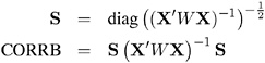
Standard errors of the estimates are computed using the equation

where is the i th diagonal element of ( X ² W X ) ^{ˆ’ 1} . The ratio

is distributed as Student s t under the hypothesis that ² _i is zero. Regression procedures display the t ratio and the significance probability, which is the probability under the hypothesis ² _i = 0 of a larger absolute t value than was actually obtained. When the probability is less than some small level, the event is considered so unlikely that the hypothesis is rejected.

Type I SS and Type II SS measure the contribution of a variable to the reduction in SSE. Type I SS measure the reduction in SSE as that variable is entered into the model in sequence. Type II SS are the increment in SSE that results from removing the variable from the full model. Type II SS are equivalent to the Type III and Type IV SS reported in the GLM procedure. If Type II SS are used in the numerator of an F test, the test is equivalent to the t test for the hypothesis that the parameter is zero. In polynomial models, Type I SS measure the contribution of each polynomial term after it is orthogonalized to the previous terms in the model. The four types of SS are described in Chapter 11, The Four Types of Estimable Functions.

Standardized estimates are defined as the estimates that result when all variables are standardized to a mean of 0 and a variance of 1. Standardized estimates are computed by multiplying the original estimates by the sample standard deviation of the regressor variable and dividing by the sample standard deviation of the dependent variable.

R ² is an indicator of how much of the variation in the data is explained by the model. It is defined as

where SSE is the sum of squares for error and TSS is the corrected total sum of squares. The Adjusted R ² statistic is an alternative to R ² that is adjusted for the number of parameters in the model. This is calculated as

where n is the number of observations used to fit the model, p is the number of parameters in the model (including the intercept), and i is 1 if the model includes an intercept term, and 0 otherwise .

Tolerances and variance inflation factors measure the strength of interrelationships among the regressor variables in the model. If all variables are orthogonal to each other, both tolerance and variance inflation are 1. If a variable is very closely related to other variables, the tolerance goes to 0 and the variance inflation gets very large. Tolerance ( TOL ) is 1 minus the R ² that results from the regression of the other variables in the model on that regressor. Variance inflation ( VIF ) is the diagonal of ( X ² W X ) ^{ˆ’ 1} if ( X ² W X ) is scaled to correlation form. The statistics are related as

Models Not of Full Rank

If the model is not full rank, then a generalized inverse can be used to solve the normal equations to minimize the SSE:

However, these estimates are not unique since there are an infinite number of solutions using different generalized inverses. PROC REG and other regression procedures choose a nonzero solution for all variables that are linearly independent of previous variables and a zero solution for other variables. This corresponds to using a generalized inverse in the normal equations, and the expected values of the estimates are the Hermite normal form of X ² W X multiplied by the true parameters:

Degrees of freedom for the zeroed estimates are reported as zero. The hypotheses that are not testable have t tests displayed as missing. The message that the model is not full rank includes a display of the relations that exist in the matrix.

Comments on Interpreting Regression Statistics

In most applications, regression models are merely useful approximations. Reality is often so complicated that you cannot know what the true model is. You may have to choose a model more on the basis of what variables can be measured and what kinds of models can be estimated than on a rigorous theory that explains how the universe really works. However, even in cases where theory is lacking, a regression model may be an excellent predictor of the response if the model is carefully formulated from a large sample. The interpretation of statistics such as parameter estimates may nevertheless be highly problematical.

Statisticians usually use the word prediction in a technical sense. Prediction in this sense does not refer to predicting the future (statisticians call that forecasting ) but rather to guessing the response from the values of the regressors in an observation taken under the same circumstances as the sample from which the regression equation was estimated. If you developed a regression model for predicting consumer preferences in 1958, it may not give very good predictions in 1988 no matter how well it did in 1958. If it is the future you want to predict, your model must include whatever relevant factors may change over time. If the process you are studying does in fact change over time, you must take observations at several, perhaps many, different times. Analysis of such data is the province of SAS/ETS procedures such as AUTOREG and STATESPACE. Refer to the SAS/ETS User s Guide for more information on these procedures.

The comments in the rest of this section are directed toward linear least-squares regression. Nonlinear regression and non-least-squares regression often introduce further complications. For more detailed discussions of the interpretation of regression statistics, see Darlington (1968), Mosteller and Tukey (1977), Weisberg (1985), and Younger (1979).

Interpreting Parameter Estimates from a Controlled Experiment

Parameter estimates are easiest to interpret in a controlled experiment in which the regressors are manipulated independently of each other. In a well-designed experiment, such as a randomized factorial design with replications in each cell , you can use lack-of-fit tests and estimates of the standard error of prediction to determine whether the model describes the experimental process with adequate precision. If so, a regression coefficient estimates the amount by which the mean response changes when the regressor is changed by one unit while all the other regressors are unchanged. However, if the model involves interactions or polynomial terms, it may not be possible to interpret individual regression coefficients. For example, if the equation includes both linear and quadratic terms for a given variable, you cannot physically change the value of the linear term without also changing the value of the quadratic term. Sometimes it may be possible to recode the regressors, for example by using orthogonal polynomials , to make the interpretation easier.

If the nonstatistical aspects of the experiment are also treated with sufficient care (including such things as use of placebos and double blinds), then you can state conclusions in causal terms; that is, this change in a regressor causes that change in the response. Causality can never be inferred from statistical results alone or from an observational study.

If the model that you fit is not the true model, then the parameter estimates may depend strongly on the particular values of the regressors used in the experiment. For example, if the response is actually a quadratic function of a regressor but you fita linear function, the estimated slope may be a large negative value if you use only small values of the regressor, a large positive value if you use only large values of the regressor, or near zero if you use both large and small regressor values. When you report the results of an experiment, it is important to include the values of the regressors. It is also important to avoid extrapolating the regression equation outside the range of regressors in the sample.

Interpreting Parameter Estimates from an Observational Study

In an observational study, parameter estimates can be interpreted as the expected difference in response of two observations that differ by one unit on the regressor in question and that have the same values for all other regressors. You cannot make inferences about changes in an observational study since you have not actually changed anything. It may not be possible even in principle to change one regressor independently of all the others. Neither can you draw conclusions about causality without experimental manipulation.

If you conduct an observational study and if you do not know the true form of the model, interpretation of parameter estimates becomes even more convoluted. A coefficient must then be interpreted as an average over the sampled population of expected differences in response of observations that differ by one unit on only one regressor. The considerations that are discussed under controlled experiments for which the true model is not known also apply.

Comparing Parameter Estimates

Two coefficients in the same model can be directly compared only if the regressors are measured in the same units. You can make any coefficient large or small just by changing the units. If you convert a regressor from feet to miles, the parameter estimate is multiplied by 5280.

Sometimes standardized regression coefficients are used to compare the effects of regressors measured in different units. Standardizing the variables effectively makes the standard deviation the unit of measurement. This makes sense only if the standard deviation is a meaningful quantity, which usually is the case only if the observations are sampled from a well-defined population. In a controlled experiment, the standard deviation of a regressor depends on the values of the regressor selected by the experimenter. Thus, you can make a standardized regression coefficient large by using a large range of values for the regressor.

In some applications you may be able to compare regression coefficients in terms of the practical range of variation of a regressor. Suppose that each independent variable in an industrial process can be set to values only within a certain range. You can rescale the variables so that the smallest possible value is zero and the largest possible value is one. Then the unit of measurement for each regressor is the maximum possible range of the regressor, and the parameter estimates are comparable in that sense. Another possibility is to scale the regressors in terms of the cost of setting a regressor to a particular value, so comparisons can be made in monetary terms.

Correlated Regressors

In an experiment, you can often select values for the regressors such that the regressors are orthogonal (not correlated with each other). Orthogonal designs have enormous advantages in interpretation. With orthogonal regressors, the parameter estimate for a given regressor does not depend on which other regressors are included in the model, although other statistics such as standard errors and p -values may change.

If the regressors are correlated, it becomes difficult to disentangle the effects of one regressor from another, and the parameter estimates may be highly dependent on which regressors are used in the model. Two correlated regressors may be nonsignificant when tested separately but highly significant when considered together. If two regressors have a correlation of 1.0, it is impossible to separate their effects.

It may be possible to recode correlated regressors to make interpretation easier. For example, if X and Y are highly correlated, they could be replaced in a linear regression by X + Y and X ˆ’ Y without changing the fit of the model or statistics for other regressors.

Errors in the Regressors

If there is error in the measurements of the regressors, the parameter estimates must be interpreted with respect to the measured values of the regressors, not the true values. A regressor may be statistically nonsignificant when measured with error even though it would have been highly significant if measured accurately.

Probability Values ( p-values )

Probability values ( p -values) do not necessarily measure the importance of a regressor. An important regressor can have a large (nonsignificant) p -value if the sample is small, if the regressor is measured over a narrow range, if there are large measurement errors, or if another closely related regressor is included in the equation. An unimportant regressor can have a very small p -value in a large sample. Computing a confidence interval for a parameter estimate gives you more useful information than just looking at the p -value, but confidence intervals do not solve problems of measurement errors in the regressors or highly correlated regressors.

The p -values are always approximations. The assumptions required to compute exact p -values are never satisfied in practice.

Interpreting R ²

R ² is usually defined as the proportion of variance of the response that is predictable from (that can be explained by) the regressor variables. It may be easier to interpret , which is approximately the factor by which the standard error of prediction is reduced by the introduction of the regressor variables.

R ² is easiest to interpret when the observations, including the values of both the regressors and response, are randomly sampled from a well-defined population. Nonrandom sampling can greatly distort R ² . For example, excessively large values of R ² can be obtained by omitting from the sample observations with regressor values near the mean.

In a controlled experiment, R ² depends on the values chosen for the regressors. A wide range of regressor values generally yields a larger R ² than a narrow range. In comparing the results of two experiments on the same variables but with different ranges for the regressors, you should look at the standard error of prediction (root mean square error) rather than R ² .

Whether a given R ² value is considered to be large or small depends on the context of the particular study. A social scientist might consider an R ² of 0.30 to be large, while a physicist might consider 0.98 to be small.

You can always get an R ² arbitrarily close to 1.0 by including a large number of completely unrelated regressors in the equation. If the number of regressors is close to the sample size , R ² is very biased . In such cases, the adjusted R ² and related statistics discussed by Darlington (1968) are less misleading.

If you fit many different models and choose the model with the largest R ² , all the statistics are biased and the p -values for the parameter estimates are not valid. Caution must be taken with the interpretation of R ² for models with no intercept term. As a general rule, no-intercept models should be fit only when theoretical justification exists and the data appear to fit a no-intercept framework. The R ² in those cases is measuring something different (refer to Kvalseth 1985).

Incorrect Data Values

All regression statistics can be seriously distorted by a single incorrect data value. A decimal point in the wrong place can completely change the parameter estimates, R ² , and other statistics. It is important to check your data for outliers and influential observations. The diagnostics in PROC REG are particularly useful in this regard.

Predicted and Residual Values

After the model has been fit, predicted and residual values are usually calculated and output. The predicted values are calculated from the estimated regression equation; the residuals are calculated as actual minus predicted. Some procedures can calculate standard errors of residuals, predicted mean values, and individual predicted values.

Consider the i th observation where x _i is the row of regressors, b is the vector of parameter estimates, and s ² is the mean squared error.

Let

where X is the design matrix for the observed data, x _i is an arbitrary regressor vector (possibly but not necessarily a row of X ), W is a diagonal matrix with the observed weights on the diagonal, and w _i is the weight corresponding to x _i .

Then

The standard error of the individual (future) predicted value y _i is

If the predictor vector x _i corresponds to an observation in the analysis data, then the residual for that observation is defined as

The ratio of the residual to its standard error, called the studentized residual , is sometimes shown as

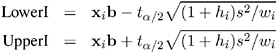
There are two kinds of confidence intervals for predicted values. One type of confidence interval is an interval for the mean value of the response. The other type, sometimes called a prediction or forecasting interval , is an interval for the actual value of a response, which is the mean value plus error.

For example, you can construct for the i th observation a confidence interval that contains the true mean value of the response with probability 1 ˆ’ ± . The upper and lower limits of the confidence interval for the mean value are

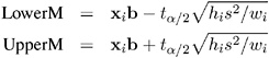
where t _{± / 2} is the tabulated t statistic with degrees of freedom equal to the degrees of freedom for the mean squared error.

The limits for the confidence interval for an actual individual response are

Influential observations are those that, according to various criteria, appear to have alargeinfluence on the parameter estimates. One measure of influence, Cook s D , measures the change to the estimates that results from deleting each observation:

where k is the number of parameters in the model (including the intercept). For more information, refer to Cook (1977, 1979).

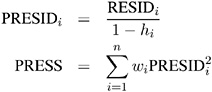
The predicted residual for observation i is defined as the residual for the i th observation that results from dropping the i th observation from the parameter estimates. The sum of squares of predicted residual errors is called the PRESS statistic :

Testing Linear Hypotheses

The general form of a linear hypothesis for the parameters is

where L is q — k , ² is k —1, and c is q —1. To test this hypothesis, the linear function is taken with respect to the parameter estimates:

This has variance

where b is the estimate of ² .

A quadratic form called the sum of squares due to the hypothesis is calculated:

If you assume that this is testable, the SS can be used as a numerator of the F test:

This is compared with an F distribution with q and df e degrees of freedom, where df e is the degrees of freedom for residual error.

Multivariate Tests

Multivariate hypotheses involve several dependent variables in the form

where L is a linear function on the regressor side, ² is a matrix of parameters, M is a linear function on the dependent side, and d is a matrix of constants. The special case (handled by PROC REG) in which the constants are the same for each dependent variable is written

where c is a column vector of constants and j is a row vector of 1s. The special case in which the constants are 0 is

These multivariate tests are covered in detail in Morrison (1976); Timm (1975); Mardia, Kent, and Bibby (1979); Bock (1975); and other works cited in Chapter 5, Introduction to Multivariate Procedures.

To test this hypothesis, construct two matrices, H and E , that correspond to the numerator and denominator of a univariate F test:

Four test statistics, based on the eigenvalues of E ^{ˆ’ 1} H or ( E + H ) ^{ˆ’ 1} H , are formed. Let » _i be the ordered eigenvalues of E ^{ˆ’ 1} H (if the inverse exists), and let ¾ _i be the ordered eigenvalues of ( E + H ) ^{ˆ’ 1} H . It happens that ¾ _i = » _i / (1 + » _i ) and » _i = ¾ _i / (1 ˆ’ ¾ _i ), and it turns out that is the i th canonical correlation.

Let p be the rank of ( H + E ), which is less than or equal to the number of columns of M . Let q be the rank of L ( X ² W X ) ˆ’ L ² . Let v be the error degrees of freedom and s = min( p, q ). Let m = ( p ˆ’ q ˆ’ 1) / 2, and let n = ( v ˆ’ p ˆ’ 1) / 2. Then the following statistics test the multivariate hypothesis in various ways, and their p-values can be approximated by F distributions. Note that in the special case that the rank of H is 1, all of these F statistics will be the same and the corresponding p-values will in fact be exact, since in this case the hypothesis is really univariate.

Wilks Lambda

If

then

is approximately F , where

The degrees of freedom are pq and rt ˆ’ 2 u . The distribution is exact if min( p, q ) ‰ 2. (Refer to Rao 1973, p. 556.)

Pillai s Trace

If

then

is approximately F with s (2 m + s +1) and s (2 n + s +1) degrees of freedom.

Hotelling-Lawley Trace

If

then for n > 0

is approximately F with pq and 4 + ( pq + 2)/( b ˆ’ 1) degrees of freedom, where b =( p + 2 n )( q + 2 n )/(2(2 n + 1)( n ˆ’ 1)) and c = (2 + ( pq + 2)/( b ˆ’ 1))/(2 n ); while for n ‰

is approximately F with s (2 m + s + 1)and 2( sn + 1)degrees of freedom.

Roy s Maximum Root

If

then

where r = max( p, q ) is an upper bound on F that yields a lower bound on the significance level. Degrees of freedom are r for the numerator and v ˆ’ r + q for the denominator.

Tables of critical values for these statistics are found in Pillai (1960).

Exact Multivariate Tests

Beginning with release 9.0 of SAS/STAT software, if you specify the MSTAT=EXACT option on the appropriate statement, p -values for three of the four tests are computed exactly (Wilks Lambda, the Hotelling-Lawley Trace, and Roy s Greatest Root), and the p -values for the fourth (Pillai s trace) are based on an F - approximation that is more accurate (but occasionally slightly more liberal ) than the default. The exact p -values for Roy s Greatest Root give an especially dramatic improvement, since in this case the F -approximation only provides a lower bound for the p -value. If you use the F -based p -value for this test in the usual way, declaring a test significant if p < . 05, then your decisions may be very liberal. For example, instead of the nominal 5% Type I error rate, such a procedure can easily have an actual Type I error rate in excess of 30%. By contrast, basing such a procedure on the exact p -values will result in the appropriate 5% Type I error rate, under the usual regression assumptions.

The exact p -values are based on the following sources:

• Wilks Lambda: Lee (1972), Davis (1979)

• Pillai s Trace: Muller (1998)

• Hotelling-Lawley Trace: Davis (1970), Davis (1980)

• Roy s Greatest Root: Davis (1972), Pillai and Flury (1984)

Note that although the MSTAT=EXACT p -value for Pillai s Trace is still approximate, it has substantially greater accuracy than the default approximation (Muller 1998).

Since most of the MSTAT=EXACT p -values are not based on the F -distribution, the columns in the multivariate tests table corresponding to this approximation ”in particular, the F value and the numerator and denominator degrees of freedom ” are no longer displayed, and the column containing the p -values is labeled P Value instead of Pr > F . Thus, for example, suppose you use the following PROC ANOVA code to perform a multivariate analysis of an archaeological data set:

  data Skulls;   input Loc . Basal Occ Max;   datalines;   Minas Graes, Brazil  2.068 2.070 1.580   Minas Graes, Brazil  2.068 2.074 1.602   Minas Graes, Brazil  2.090 2.090 1.613   Minas Graes, Brazil  2.097 2.093 1.613   Minas Graes, Brazil  2.117 2.125 1.663   Minas Graes, Brazil  2.140 2.146 1.681   Matto Grosso, Brazil 2.045 2.054 1.580   Matto Grosso, Brazil 2.076 2.088 1.602   Matto Grosso, Brazil 2.090 2.093 1.643   Matto Grosso, Brazil 2.111 2.114 1.643   Santa Cruz, Bolivia  2.093 2.098 1.653   Santa Cruz, Bolivia  2.100 2.106 1.623   Santa Cruz, Bolivia  2.104 2.101 1.653   ;   proc anova data=Skulls;   class Loc;   model Basal Occ Max = Loc / nouni;   manova h=Loc;   ods select MultStat;   run;  

The default multivariate tests, based on the F -approximations, are shown in Figure 2.3.

  The ANOVA Procedure   Multivariate Analysis of Variance   MANOVA Test Criteria and F Approximations for   the Hypothesis of No Overall Loc Effect   H = Anova SSCP Matrix for Loc   E = Error SSCP Matrix   S=2    M=0    N=3   Statistic                        Value    F Value    Num DF    Den DF    Pr > F   Wilks' Lambda               0.60143661       0.77         6        16    0.6032   Pillai's Trace              0.44702843       0.86         6        18    0.5397   Hotelling-Lawley Trace      0.58210348       0.75         6    9.0909    0.6272   Roy's Greatest Root         0.35530890       1.07         3         9    0.4109   NOTE: F Statistic for Roy's Greatest Root is an upper bound.   NOTE: F Statistic for Wilks' Lambda is exact.  

Figure 2.3: Default Multivariate Tests

If you specify MSTAT=EXACT on the MANOVA statement

  proc anova data=Skulls;   class Loc;   model Basal Occ Max = Loc / nouni;   manova h=Loc / mstat=exact;   ods select MultStat;   run;  

then the displayed output is the much simpler table shown in Figure 2.4.

  The ANOVA Procedure   Multivariate Analysis of Variance   MANOVA Tests for the Hypothesis of No Overall Loc Effect   H = Anova SSCP Matrix for Loc   E = Error SSCP Matrix   S=2    M=0    N=3   Statistic                        Value    P-Value   Wilks' Lambda               0.60143661     0.6032   Pillai's Trace              0.44702843     0.5521   Hotelling-Lawley Trace      0.58210348     0.6337   Roy's Greatest Root         0.35530890     0.7641  

Figure 2.4: Multivariate Tests with MSTAT=EXACT

Notice that the p -value for Roy s Greatest Root is substantially larger in the new table, and correspondingly more in line with the p -values for the other tests.

If you reference the underlying ODS output object for the table of multivariate statistics, it is important to note that its structure does not depend on the value of the MSTAT= specification. In particular, it always contains columns corresponding to both the default MSTAT=FAPPROX and the MSTAT=EXACT tests. Moreover, since the MSTAT=FAPPROX tests are relatively cheap to compute, the columns corresponding to them are always filled in, even though they are not displayed when you specify MSTAT=EXACT. On the other hand, for MSTAT=FAPPROX (which is the default), the column of exact p -values contains missing values, and is not displayed.