Auditing Workbooks

The auditing features are some of the most useful tools in Excel. These tools can help you detect problems in your worksheet formulas. Excel supplies a Formula Auditing toolbar to help you find errors on your worksheets, attach comments to cells , and track problems in your worksheet formulas.

Using auditing tools can help you understand, visualize, and troubleshoot the relationships among cell references, formulas, and data.

When you're auditing formulas in your worksheets, you might want to use the Go To Special command to quickly search for comments, precedents , dependents, or any other auditing information. The Go To Special command helps you find the following information while auditing your worksheets:

• Comments

• Constants

• Formulas that meet particular criteria

• Blank cells

• Cells in the current region or array

• Cells that do not fit a pattern in a row or column

• Precedents

• Dependents

• Last active cell in your sheet

• Visible cells

• Objects

To use the Go To Special command, simply press F5 (Go To) and click the Special button in the Go To dialog box. In the Go To Special dialog box, select the item you want to go to and click OK. Excel highlights the cells on the worksheet that correspond to the item you selected in the Go To Special dialog box.

Understanding Dependents and Precedents

Before you audit a worksheet, you should be familiar with the following auditing terms:

• Constant Cells with contents that are that are used by other cells that contain formulas. In Excel, cells containing values that do not begin with an equal sign are constants, whether they are numbers or text.

• Dependent Cells that contain formulas that refer to other cells.

• Error Values that result from an incorrect cell reference or formula.

• Precedent Cells that are referred to directly by a formula.

• Tracer A visual tool that enables you to find precedents, dependents, and errors in any cell in a worksheet. Tracers are graphic displays, such as arrows, that visually show you where formulas get their values. Tracers show relationships between cells and illustrate precedent and dependent relationships.

Using the Formula Auditing Toolbar

Excel's Formula Auditing toolbar provides tools for auditing data in your worksheets. Figure 16.1 shows the Formula Auditing toolbar. To display the Formula Auditing toolbar, choose Tools, Formula Auditing, Show Formula Auditing Toolbar.

Figure 16.1. The Formula Auditing toolbar.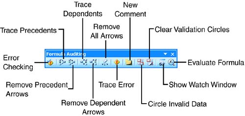

Table 16.1 lists the auditing tools on the Formula Auditing toolbar and describes the purpose of each tool.

Table 16.1. Excel's Auditing Tools

Tool	What It Does
Error Checking	Checks for problems in formulas on the worksheet using a set of rules to find common mistakes.
Trace Precedents	Draws arrows from all cells that supply values directly to the formula in the active cell (precedents).
Remove Precedent Arrows	Deletes a level of precedent tracer arrows from the active worksheet.
Trace Dependents	Draws arrows from the active cell to cells with formulas that use the values in the active cell (dependents).
Remove Dependent Arrows	Deletes a level of dependent tracer arrows from the active worksheet.
Remove All Arrows	Deletes all tracer arrows from the active worksheet.
Trace Error	Draws an arrow to an error value in the active cell from cells that might have caused the error.
New Comment	Displays a comment text box next to a cell you selected that will contain text or audio comments.
Circle Invalid Data	Identifies incorrect entries with circles. Incorrect entries are values outside the limits you set by using the Data Validation command.
Clear Validation Circles	Hides circles around incorrect values in cells.
Show Watch Window	Displays the Watch Window toolbar, allowing you to watch cells and their formulas, even when the cells are not in view.
Evaluate Formula	Displays the parts of a nested formula, which tests cell contents and helps you make decisions based upon the results. Evaluates the order in which the nested formula is calculated.

Using Error Checking

The Error Checking feature checks formulas for problems using a set of rules to find common mistakes. Error checking is similar to spelling checker and grammar checker in that rules are used and not find all errors are found.

You can turn the error checking rules on or off individually. To do so, choose Tools, Options, and click the Error Checking tab (see figure 16.2). By default, background error checking is turned on. That way, Excel immediately checks for formula errors on the worksheet as you work. If you choose to turn off the background error-checking feature, you can check for formula errors one at a time like a spelling checker.

Figure 16.2. The Error Checking tab in the Options dialog box.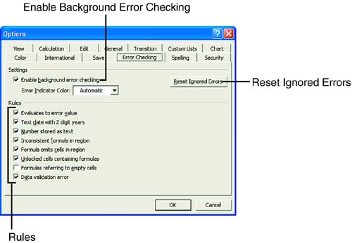

Another error checking option is to reset all previously ignored errors so that they appear again. To set this option, click the Reset Ignored Errors button. Select the rules you want to turn on or off and click OK.

When Excel finds a problem with a formula, a green triangle appears in the upper left corner of the cell that contains the formula.

If you turned off background error checking and decide to check for errors in formulas manually, click the Error Checking button on the Formula Editing toolbar and Excel will display the green triangle in the cell with the problem.

When error checking finds a formula with a problem, you should see options for resolving the problem. You can either select one of the options or ignore the problem. If you ignore a problem, it does not appear in subsequent error checks.

Using Tracer Arrows

When you audit a worksheet to trace the precedents or dependents of a cell, Excel displays the following tracer arrow symbols on your worksheet:

• Blue or solid arrow Indicates direct precedents of the selected formula.

• Red or dotted arrow Indicates formulas that refer to error values.

• Dashed arrow attached to a spreadsheet icon Refers to external worksheets.

Before you use tracer arrows to audit your worksheet, you need to verify that the Hide All option is not selected in the Options dialog box. When the Hide All option is not selected, Excel displays the tracer arrows on your worksheets. If the option is selected, Excel does not display any tracer arrows when you audit your worksheets.

To verify that the Hide All option is turned off, choose Tools, Options. In the Options dialog box, click the View tab if necessary. In the Objects section, verify that the Hide All option button is not selected and that the Show All option button is selected (displays with a black circle in the radio button), as shown in Figure 16.3. Click OK. Now you're all set to audit your worksheet using tracer arrows.

Figure 16.3. The Show All option in the Options dialog box.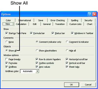

Go through the steps in the next To Do exercise to trace precedents and dependents with tracer arrows. The first step is to display the Formula Auditing toolbar. You need to work with the My Budget workbook for the entire hour , so be sure to open it before you start the exercise. If you are prompted to update linked information, choose Yes.

To Do: Trace Precedents Using Tracer Arrows

1. Choose Tools, Formula Auditing, Show Formula Auditing Toolbar. Excel displays the Formula Auditing toolbar.

2. To trace the precedents of a cell (to figure out the relationship between a formula and its cell references), click the cell that contains the formula you want to trace. In this case, click cell B9.

3. Click the Trace Precedents button on the Formula Auditing toolbar. Excel displays a tracer arrow on the worksheet, as shown in Figure 16.4.

   Figure 16.4. A precedent tracer arrow on the worksheet.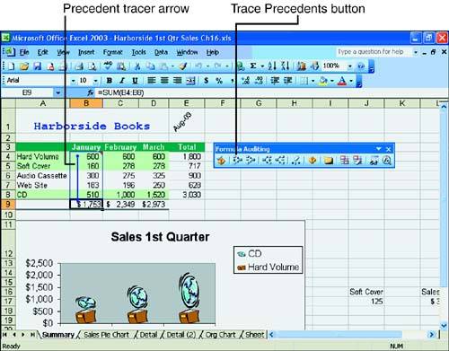

   

4. Double-click the point of the tracer arrow (blue or solid arrow) to select the cells leading up to the cell at the point end of the arrow. The cells that are referenced in the formula are highlighted.

5. Double-click the point of the tracer arrow again to select the cell at the point end of the arrow. Excel removes the highlighting from the cells related to the formula.

6. Click cell J17. This cell contains the formula you want to trace.

7. Click the Trace Precedents button on the Formula Auditing toolbar. Excel displays a tracer arrow on the worksheet.

8. Double-click the point of the external worksheet arrow (dashed arrow with a spreadsheet icon). The Go To dialog box opens (see Figure 16.5).

   Figure 16.5. The Go To dialog box.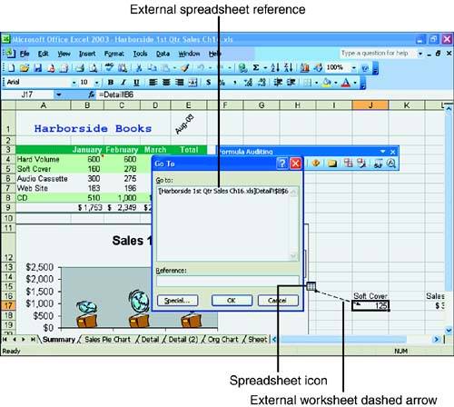

   

9. Select the item in the Go To list. Excel displays the spreadsheet reference in the Reference box at the bottom of the dialog box. Click OK to confirm your choice. Excel should display the selected sheet (Detail sheet tab) and make cell B5 the active cell. The active cell references the formula you're tracing.

10. Click the Summary sheet tab to return to the original worksheet.

11. Click the Remove Precedents Arrows button on the Formula Auditing toolbar to remove one level of tracer arrows. The external spreadsheet tracer arrow and spreadsheet icon should disappear.

The next exercise shows you how to trace dependents with tracer arrows to determine the relationship between a cell reference and the formula that contains the cell reference. You should be using the Detail worksheet.

To Do: Trace Dependents Using Tracer Arrows

1. Click the cell dependent that you want to trace. In this case, click cell B5.

2. Click the Trace Dependents button on the Formula Auditing toolbar. Excel displays tracer arrows on the worksheet, as shown in Figure 16.6.

   Figure 16.6. Dependent tracer arrows on the worksheet.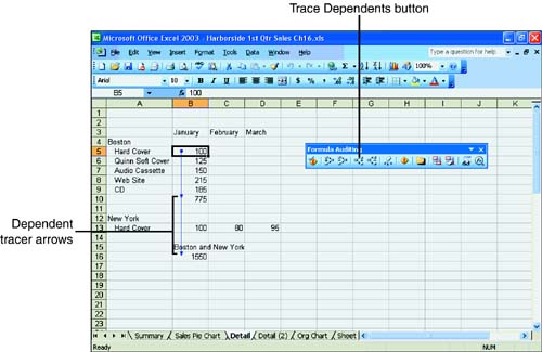

   

3. Double-click the point of the tracer arrow (blue or solid arrow) that points to cell B10 to select the cell at the point end of the arrow. The active cell is now B10.

4. Double-click the point of the tracer arrow again to select the cell at the opposite end of the arrow. The active cell is B5.

5. Double-click the point of the tracer arrow (blue or solid arrow) that points to cell C23 to select the cell at the point end of the arrow. The active cell is now C23.

6. Double-click the point of the tracer arrow again to select the cell at the opposite end of the arrow. The active cell is B5.

7. Click the Remove Dependent Arrows button on the Formula Auditing toolbar to remove the tracer arrows.

Tracing Errors

After tracing precedents and dependents, you can also trace any errors in your worksheet. If you have formulas that produce errors, Excel's Trace Errors feature can help you find and correct the errors.

Tracing errors in a worksheet pinpoints the errors so that you can fix them. Some of the error values that can appear in a cell include the following:

• #DIV/0! Occurs when you create a formula that divides by zero ( ) or divides by a cell that is empty.

• #N/A Happens when you have a value that is not available to a function or a formula.

• # NAME ? Appears when Excel doesn't recognize text in a formula.

• #NULL! Happens when you specify an intersection of two areas that do not intersect. For instance, you might have an incorrect range operator (not using a comma to separate two ranges, such as =SUM(B1:B8,F4:F8 ) or an incorrect cell reference.

• #NUM! Occurs when you use an unacceptable argument in a function that should be a numeric argument or when a formula's result is a number that is too large or too small for Excel to display. Excel displays values between -1*10307 and 1*10307 .

• #REF! Happens when a cell reference is not valid, such as when you delete cells that refer to formulas or paste cells onto cells that are referred to by other formulas.

• #VALUE! Appears when you use the wrong type of argument in a function or wrong operand in a formula.

The following To Do exercise walks you through tracing an error that appears in a cell. First you introduce an error by editing a formula to get incorrect results. (Continue working in the Detail worksheet.)

To Do: Trace Errors

1. Click cell B10, press F2, and press the End key. Next, type / , click B4, and press Enter. You should see the #DIV/0! error in cell B10. This error value is traceable .

2. Select cell B10 and click the Trace Error button on the Formula Auditing toolbar. Excel displays an error tracer arrow on the worksheet, as shown in Figure 16.7. You should also see a Trace Error icon (diamond with an exclamation point) next to cell B10. If you point to the Trace Error icon, a ScreenTip informs you that the formula or function is dividing by zero or empty cells.

   Figure 16.7. An error tracer arrow on the worksheet.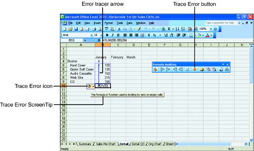

   

   

   If you click on the Trace Error down arrow, you will see a shortcut menu with commands for fixing the formula error.

   
   

3. Double-click the point of the error tracer arrow (red, dotted, blue, or solid arrow) to select the cell at the base of the arrow. The active cell is B4, which is the cause of the error. Cell B4 is empty, which means the cell has a value of zero ( ). Zero cannot be a divisor, and you cannot divide by zero. Therefore, Excel displayed the #DIV/0! error result in cell B10.

4. Double-click the point of the error tracer arrow again to select the cell at the point end of the arrow. Cell B10 is the active cell.

5. In cell B10, type =SUM(B5:B9) to correct the error. Press Enter. The error tracer arrow should disappear.

   

   If you correct an error and the little green triangle doesn't disappear, it doesn't mean you didn't fix the error correctlyit means you have another error to clear.

   
   

6. Click the Close ( x ) button on the Formula Auditing toolbar to close the toolbar.