44. | C++ Neural Networks and Fuzzy Logic

C++ Neural Networks and Fuzzy Logic
by Valluru B. Rao
M&T Books, IDG Books Worldwide, Inc.
ISBN: 1558515526 Pub Date: 06/01/95

Table of Contents

Delta Rule

The delta rule is also known as the least mean squared error rule (LMS). You first calculate the square of the errors between the target or desired values and computed values, and then take the average to get the mean squared error. This quantity is to be minimized. For this, realize that it is a function of the weights themselves, since the computation of output uses them. The set of values of weights that minimizes the mean squared error is what is needed for the next cycle of operation of the neural network. Having worked this out mathematically, and having compared the weights thus found with the weights actually used, one determines their difference and gives it in the delta rule, each time weights are to be updated. So the delta rule, which is also the rule used first by Widrow and Hoff, in the context of learning in neural networks, is stated as an equation defining the change in the weights to be affected.

Suppose you fix your attention to the weight on the connection between the ith neuron in one layer and the jth neuron in the next layer. At time t, this weight is w_ij(t) . After one cycle of operation, this weight becomes w_ij(t + 1). The difference between the two is w_ij(t + 1) - w_ij(t), and is denoted by [Delta]w_ij . The delta rule then gives [Delta]w_ij as :

 [Delta]w_ij = 2[mu]x_i(desired output value – computed output value)_j

Here, [mu] is the learning rate, which is positive and much smaller than 1, and x_i is the ith component of the input vector.

Supervised Learning

Supervised neural network paradigms to be discussed include :

• Perceptron

• Adaline

• Feedforward Backpropagation network

• Statistical trained networks (Boltzmann/Cauchy machines)

• Radial basis function networks

The Perceptron and the Adaline use the delta rule; the only difference is that the Perceptron has binary output, while the Adaline has continuous valued output. The Feedforward Backpropagation network uses the generalized delta rule, which is described next.

Generalized Delta Rule

While the delta rule uses local information on error, the generalized delta rule uses error information that is not local. It is designed to minimize the total of the squared errors of the output neurons. In trying to achieve this minimum, the steepest descent method, which uses the gradient of the weight surface, is used. (This is also used in the delta rule.) For the next error calculation, the algorithm looks at the gradient of the error surface, which gives the direction of the largest slope on the error surface. This is used to determine the direction to go to try to minimize the error. The algorithm chooses the negative of this gradient, which is the direction of steepest descent. Imagine a very hilly error surface, with peaks and valleys that have a wide range of magnitude. Imagine starting your search for minimum error at an arbitrary point. By choosing the negative gradient on all iterations, you eventually end up at a valley. You cannot know, however, if this valley is the global minimum or a local minimum. Getting stuck in a local minimum is one well-known potential problem of the steepest descent method. You will see more on the generalized delta rule in the chapter on backpropagation (Chapter 7).

Statistical Training and Simulated Annealing

The Boltzmann machine (and Cauchy machine) uses probabilities and statistical theory, along with an energy function representing temperature. The learning is probabilistic and is called simulated annealing. At different temperature levels, a different number of iterations in processing are used, and this constitutes an annealing schedule. Use of probability distributions is for the goal of reaching a state of global minimum of energy. Boltzmann distribution and Cauchy distribution are probability distributions used in this process. It is obviously desirable to reach a global minimum, rather than settling down at a local minimum.

Figure 6.1 clarifies the distinction between a local minimum and a global minimum. In this figure you find the graph of an energy function and points A and B. These points show that the energy levels there are smaller than the energy levels at any point in their vicinity, so you can say they represent points of minimum energy. The overall or global minimum, as you can see, is at point B, where the energy level is smaller than that even at point A, so A corresponds only to a local minimum. It is desirable to get to B and not get stopped at A itself, in the pursuit of a minimum for the energy function. If point C is reached, one would like the further movement to be toward B and not A. Similarly, if a point near A is reached, the subsequent movement should avoid reaching or settling at A but carry on to B. Perturbation techniques are useful for these considerations.

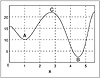
Figure 6.1 Local and global minima.

Clamping Probabilities

Sometimes in simulated annealing, first a subset of the neurons in the network are associated with some inputs, and another subset of neurons are associated with some outputs, and these are clamped with probabilities, which are not changed in the learning process. Then the rest of the network is subjected to adjustments. Updating is not done for the clamped units in the network. This training procedure of Geoffrey Hinton and Terrence Sejnowski provides an extension of the Boltzmann technique to more general networks.

Radial Basis-Function Networks

Although details of radial basis functions are beyond the scope of this book, it is worthwhile to contrast the learning characteristics for this type of neural network model. Radial basis-function networks in topology look similar to feedforward networks. Each neuron has an output to input characteristic that resembles a radial function (for two inputs, and thus two dimensions). Specifically, the output h(x) is as follows:

 h(x)  = exp [ (x - u)² / 2[sigma]²   ]

Here, x is the input vector, u is the mean, and [sigma] is the standard deviation of the output response curve of the neuron. Radial basis function (RBF) networks have rapid training time (orders of magnitude faster than backpropagation) and do not have problems with local minima as backpropagation does. RBF networks are used with supervised training, and typically only the output layer is trained. Once training is completed, a RBF network may be slower to use than a feedforward Backpropagation network, since more computations are required to arrive at an output.

Table of Contents