Measuring IP Network Performance

This section outlines some of the available data on IP network performance, including published results on average packet loss, patterns of loss, packet corruption and duplication, transit time, and the effects of multicast.

Several studies have measured network behavior over a wide range of conditions on the public Internet. For example, Paxson reports on the behavior of 20,000 transfers among 35 sites in 9 countries ; ^{124 , 95} Handley ¹²² and Bolot ^{67 , 66} report on the behavior of multicast sessions; and Yajnik, Moon, Kurose, and Towsley report on the temporal dependence in packet loss statistics. ⁸⁹ , ¹⁰⁸ , ¹⁰⁹ Other sources of data include the traffic archives maintained by CAIDA (the Cooperative Association for Internet Data Analysis), ¹¹⁷ the NLANR (National Laboratory for Applied Network Research), ¹¹⁹ and the ACM (Association for Computing Machinery). ¹¹⁶

Average Packet Loss

Various packet loss metrics can be studied. For example, the average loss rate gives a general measure of network congestion, while loss patterns and correlation give insights into the dynamics of the network.

The reported measurements of average packet loss rate show a range of conditions. For example, measurements of TCP/IP traffic taken by Paxson in 1994 and 1995 show that 30% to 70% of flows, depending on path taken and date, showed no packet loss, but of those flows that did show loss, the average loss ranged from 3% to 17% (these results are summarized in Table 2.1). Data from Bolot, using 64-kilobit PCM-encoded audio, shows similar patterns, with loss rates between 4% and 16% depending on time of day, although this data also dates from 1995. More recent results from Yajnik et al., taken using simulated audio traffic in 1997 “1998, show lower loss rates of 1.38% to 11.03%. Handley's results ”two sets of approximately 3.5 million packets of data and reception report statistics for multicast video sessions in May and September 1996 ”show loss averaged over five-second intervals varying between 0% and 100%, depending on receiver location and time of day. A sample for one particular receiver during a ten- hour period on May 29, 1996, plotted in Figure 2.5, shows the average loss rate, sampled over five-second intervals, varying between 0% and 20%.

Figure 2.5. Loss Rate Distribution versus Time ¹²²

Table 2.1. Packet Loss Rates for Various Regions ⁹⁵

	Fraction of Flows Showing No Loss		Average Loss Rate for Flows with Loss
Region	Dec. 1994	Dec. 1995	Dec. 1994	Dec. 1995
Within Europe	48%	58%	5.3%	5.9%
Within U.S.	66%	69%	3.6%	4.4%
U.S. to Europe	40%	31%	9.8%	16.9%
Europe to U.S.	35%	52%	4.9%	6.0%

The observed average loss rate is not necessarily constant, nor smoothly varying. The sample shows a loss rate that, in general, changes relatively smoothly, although at some points a sudden change occurs. Another example, from Yajnik et al., is shown in Figure 2.6. This case shows a much more dramatic change in loss rate: After a slow decline from 2.5% to 1% over the course of one hour, the loss rate jumps to 25% for 10 minutes before returning to normal ”a process that repeats a few minutes later.

Figure 2.6. Loss Rate Distribution versus Time (Adapted from M. Yajnik, S. Moon, J. Kurose, and D. Towsley, "Measurement and Modeling of the Temporal Dependence in Packet Loss," Technical Report 98-78, Department of Computer Science, University of Massachusetts, Amherst, 1998. 1999 IEEE.)

How do these loss rates compare with current networks? The conventional wisdom at the time of this writing is that it's possible to engineer the network backbone such that packet loss never occurs, so one might expect recent data to illustrate this. To some extent this is true; however, even if it's possible to engineer part of the network to be loss free, that possibility does not imply that the entire network will behave in the same way. Many network paths show loss today, even if that loss represents a relatively small fraction of packets.

The Internet Weather Report, ¹²⁰ a monthly survey of the loss rate measured in a range of routes across the Internet, showed average packet loss rates within the United States ranging from 0% to 16%, depending on the ISP, as of May 2001. The monthly average loss rate is about 2% in the United States, but for the Internet as a whole, the average is slightly higher, at about 3%.

What should we learn from this? Even though some parts of the network are well engineered, others can show significant loss. Remember, as Table 2.1 shows, 70% of network paths within the United States had no packet loss in 1995, yet the average loss rate for the others was almost 5%, a rate that is sufficient to cause significant degradation in audio/video quality.

Packet Loss Patterns

In addition to looking at changes in the average loss rate, it is instructive to consider the short- term patterns of loss. If we aim to correct for packet loss, it helps to know if lost packets are randomly distributed within a media flow, or if losses occur in bursts.

If packet losses are distributed uniformly in time, we should expect that the probability that a particular packet is lost is the same as the probability that the previous packet was lost. This would mean that packet losses are most often isolated events, a desirable outcome because a single loss is easier to recover from than a burst. Unfortunately, however, the probability that a particular packet is lost often increases if the previous packet was also lost. That is, losses tend to occur back-to-back. Measurements by Vern Paxson have shown, in some cases, a five- to tenfold increase in loss probability for a particular packet if the previous packet was lost, clearly implying that packet loss is not uniformly distributed in time.

Several other studies ”for example, measurements collected by Bolot in 1995, by Handley and Yajnik et al. in 1996, and by me in 1999 ”have confirmed the observation that packet loss probabilities are not independent. In all cases, these studies show that the vast majority of losses are of single packets, constituting about 90% of loss events. The probability of longer bursts of loss decreases as illustrated in Figure 2.7; it is clear that longer bursts occur more frequently than they would if losses were independent.

Figure 2.7. Frequency Distribution of the Number of Consecutively Lost Packets

Observed loss patterns also show significant periodicity in some cases. For example, Handley has reported bursts of loss occurring approximately every 30 seconds on measurements taken in 1996 (see Figure 2.8), and similar problems were reported in April 2001. ¹²¹ Such reports are not universal, and many traces show no such effect. It is conjectured that the periodicity is due to the overloading of certain systems by routing updates, but this is not certain.

Figure 2.8. Autocorrelation of Packet Loss

Packet Duplication

If packets can be lost in the network, can they be duplicated ? Perhaps surprisingly, the answer is yes! It is possible for a source to send a single packet, yet for the receiver to get multiple copies of that packet. The most likely reason for duplication is faults in routing/switching elements within the network; duplication should not happen in normal operation.

How common is duplication? Paxson's measurements revealing the tendency of back-to-back packet losses also showed a small amount of packet duplication. In measuring 20,000 flows, he found 66 duplicate packets, but he also noted, "We have observed traces . . . in which more than 10% of the packets were replicated. The problem was traced to an improperly configured bridging device." ⁹⁵ A trace that I took in August 1999 shows 131 duplicates from approximately 1.25 million packets.

Packet duplication should not cause problems, as long as applications are aware of the issue and discard duplicates (RTP contains a sequence number for this purpose). Frequent packet duplication wastes bandwidth and is a sign that the network contains badly configured or faulty equipment.

Packet Corruption

Packets can be corrupted, as well as lost or duplicated. Each IP packet contains a checksum that protects the integrity of the packet header, but the payload is not protected at the IP layer. However, the link layer may provide a checksum, and both TCP and UDP enable a checksum of the entire packet. In theory, these protocols will detect most corrupted packets and cause them to be dropped before they reach the application.

Few statistics on the frequency of packet corruption have been reported. Stone ¹⁰³ quotes Paxson's observation that approximately one in 7,500 packets failed their TCP or UDP checksum, indicating corruption of the packet. Other measurements in that work show average checksum failure rates ranging from one in 1,100 to one in 31,900 packets. Note that this result is for a wired network; wireless networks can be expected to have significantly different properties because corruption due to radio interference may be more severe than that due to noise in wires.

When the checksum fails, the packet is assumed to be corrupted and is discarded. The application does not see corrupted packets; they appear to be lost. Corruption is visible as a small increase in the measured loss rate.

In some cases it may be desirable for an application to receive corrupt packets, or to get an explicit indication that the packets are corrupted. UDP provides a means of disabling the checksum for these cases. Chapter 8, Error Concealment, and Chapter 10, Congestion Control, discuss this topic in more detail.

Network Transit Time

How long does it take packets to transit the network? The answer depends on the route taken, and although a short path does take less time to transit than a long one, we need to be careful of the definition of short .

The components that affect transit time include the speed of the links, the number of routers through which a packet must pass, and the amount of queuing delay imposed by each router. A path that is short in physical distance may be long in the number of hops a packet must make, and often the queuing delay in the routers at each hop is the major factor. In network terms a short path is most often the one with the least hops, even if it covers a longer physical distance. Satellite links are the obvious exception, where distance introduces a significant radio propagation delay. Some measures of average round-trip time, taken in May 2001, are provided in Table 2.2 for comparison. Studies of telephone conversations subject to various round-trip delays have shown that people don't notice delays of less than approximately 300 milliseconds (ms). Although this is clearly a subjective measurement, dependent on the person and the task, the key point is that the measured network round-trip times are mostly within this limit. (The trip from London to Sydney is the exception, but the significant increase here is probably due to a satellite hop in the path.)

Table 2.2. Sample Round-Trip Time Measurements

Source	Destination	Hop Count	Round-Trip Time (ms)
Washington, DC	London	20	94
Washington, DC	Berkeley, CA	21	88
London	Berkeley, CA	22	136
London	Sydney	28	540

Measures of the delay in itself are not very interesting because they so clearly depend on the location of the source and the destination. Of more interest is how the network transit time varies from packet to packet: A network that delivers packets with constant delay is clearly easier for an application to work with than one in which the transit time can vary, especially if that application has to present time-sensitive media.

A crude measure of the variation in transit time ( jitter ) is the arrival rate of packets. For example, Figure 2.9 shows the measured arrival rate for a stream sent at a constant rate; clearly the arrival rate varies significantly, indicating that the transit time across the network is not constant.

Figure 2.9. The Packet Arrival Rate

A better measure, which doesn't assume constant rate, is to find the transit time by measuring the difference between arrival time and departure time for each packet. Unfortunately, measuring the absolute transit time is difficult because it requires accurate synchronization between the clocks at source and destination, which is not often possible. As a result, most traces of network transit time include the clock offset, and it becomes impossible to study anything other than the variation in delay (because it is not possible to determine how much of the offset is due to unsynchronized clocks and how much is due to the network).

Some sample measurements of the variation in transit time, including the offset due to unsynchronized clocks, are presented in Figure 2.10 and Figure 2.11. I took these measurements in August 1999; similar measurements have been presented by Ramjee et al. (in 1994) ⁹⁶ and by Moon et al. ⁹⁰ Note the following:

• The slow downward slope of the measurements is due to clock skew between the source and the destination. One machine's clock is running slightly faster than the other's, leading to a gradual change in the perceived transit time.

• Several step changes in the average transit time, perhaps due to route changes in the network, can be observed.

• The transit time is not constant; rather it shows significant variation throughout the session.

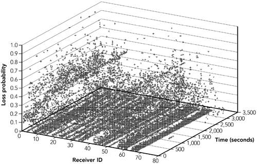
Figure 2.10. Variation in Network Transit Time: 400-Second Sample

Figure 2.11. Variation in Network Transit Time: 10-Second Sample

These are all problems that an application, or higher-layer protocol, must be prepared to handle and, if necessary, correct.

It is also possible for packets to be reordered within the network ”for example, if the route changes and the new route is shorter. Paxson ⁹⁵ observed that a total 2% of TCP data packets were delivered out of order, but that the fraction of out-of-order packets varied significantly between traces, with one trace showing 15% of packets being delivered out of order.

Another characteristic that may be observed is "spikes" in the network transit time, such as those shown in Figure 2.12. It is unclear whether these spikes are due to buffering within the network or in the sending system, but they present an interesting challenge if one is attempting to smooth the arrival time of a sequence of packets.

Figure 2.12. Spikes in Network Transit Time (Adapted from Moon et al., 1998). ⁹¹

Finally, the network transit time can show periodicity (as noted, for example, in Moon et al. 1998 ⁸⁹ ), although this appears to be a secondary effect. We expect this periodicity to have causes similar to those of the loss periodicity noted earlier, except that the events are less severe and cause queue buildup in the routers, rather than queue overflow and hence packet loss.

Acceptable Packet Sizes

The IP layer can accept variably sized packets, up to 65,535 octets in length, or to a limit determined by the maximum transmission unit (MTU) of the links traversed. The MTU is the size of the largest packet that can be accommodated by a link. A common value is 1,500 octets, which is the largest packet an Ethernet can deliver. Many applications assume that they can send packets up to this size, but some links have a lower MTU. For example, it is not unusual for dial-up modem links to have an MTU of 576 octets.

In most cases the bottleneck link is adjacent to either sender or receiver. Virtually all backbone network links have an MTU of 1,500 octets or more.

IPv4 supports fragmentation, in which a large packet is split into smaller fragments when it exceeds the MTU of a link. It is generally a bad idea to rely on this, though, because the loss of any one fragment will make it impossible for the receiver to reconstruct the packet. The resulting loss multiplier effect is something we want to avoid.

In virtually all cases, audio packets fall within the network MTU. Video frames are larger, and applications should split them into multiple packets for transport so that each packet fits within the MTU of the network.

Effects of Multicast

IP multicast enables a sender to transmit data to many receivers at the same time. It has the useful property that the network creates copies of the packet as needed, such that only one copy of the packet traverses each link. IP multicast provides for extremely efficient group communication, provided it is supported by the network, making the cost of sending data to a group of receivers independent of the size of the group .

Support for multicast is an optional, and relatively new, feature of IP networks. At the time of this writing, it is relatively widely deployed in research and educational environments and in the network backbone, but it is uncommon in many commercial settings and service providers.

Sending to a group means that more things can go wrong: Reception quality is no longer affected by a single path through the network, but by the path from the source to each individual receiver. The defining factor in the measurement of loss and delay characteristics for a multicast session is heterogeneity . Figure 2.13 illustrates this concept, showing the average loss rate seen at each receiver in a multicast session measured by me.

Figure 2.13. Loss Rates in a Multicast Session

Multicast does not change the fundamental causes of loss or delay in the network. Rather it enables each receiver to experience those effects while the source transmits only a single copy of each packet. The heterogeneity of the network makes it difficult for the source to satisfy all receivers: Sending too fast for some and too slow for others is common. We will discuss these issues further in later chapters. For now it's sufficient to note that multicast adds yet more heterogeneity to the system.

Effects of Network Technologies

The measurements that have been presented so far have been of the public, wide area, Internet. Many applications will operate in this environment, but a significant number will be used in private intranets , on wireless networks, or on networks that support enhanced quality of service. How do such considerations affect the performance of the IP layer?

Many private IP networks (often referred to as intranets ) have characteristics very similar to those of the public Internet: The traffic mix is often very similar, and many intranets cover wide areas with varying link speeds and congestion levels. In such cases it is highly likely that the performance will be similar to that measured on the public Internet. If, however, the network is engineered specifically for real-time multimedia traffic, it is possible to avoid many of the problems that have been discussed and to build an IP network that has no packet loss and minimal jitter.

Some networks support enhanced quality of service (QoS) using, for example, integrated services/RSVP ¹¹ or differentiated services. ²⁴ The use of enhanced QoS may reduce the need for packet loss and/or jitter resilience in an application because it provides a strong guarantee that certain performance bounds are met. Note, however, that in many cases the guarantee provided by the QoS scheme is statistical in nature, and often it does not completely eliminate packet loss, or perhaps more commonly, variations in transit time.

Significant performance differences can be observed in wireless networks. For example, cellular networks can exhibit significant variability in their performance over short time frames, including noncongestive loss, bursts of loss, and high bit error rates. In addition, some cellular systems have high latency because they use interleaving at the data link layer to hide bursts of loss or corruption.

The primary effect of different network technologies is to increase the heterogeneity of the network. If you are designing an application to work over a restricted subset of these technologies, you may be able to leverage the facilities of the underlying network to improve the quality of the connection that your application sees. In other cases the underlying network may impose additional challenges on the designer of a robust application.

A wise application developer will choose a robust design so that when an application moves from the network where it was originally envisioned to a new network, it will still operate correctly. The challenge in designing audiovisual applications to operate over IP is making them reliable in the face of network problems and unexpected conditions.

Conclusions about Measured Characteristics

Measuring, predicting, and modeling network behavior are complex problems with many subtleties. This discussion has only touched on the issues, but some important conclusions are evident.

The first point is that the network can and frequently does behave badly. An engineer who designs an application that expects all packets to arrive , and to do so in a timely manner, will have a surprise when that application is deployed on the Internet. Higher-layer protocols ”such as TCP ”can hide some of this badness, but there are always some aspects visible to the application.

Another important point to recognize is the heterogeneity in the network. Measurements taken at one point in the network will not represent what's happening at a different point, and even "unusual" events happen all the time. There were approximately 100 million systems on the Net at the end of 2000, ¹¹⁸ so even an event that occurs to less than 1% of hosts will affect many hundreds of thousands of machines. As an application designer, you need to be aware of this heterogeneity and its possible effects.

Despite this heterogeneity, an attempt to summarize the discussion of loss and loss patterns reveals several "typical" characteristics:

• Although some network paths may not exhibit loss, these paths are not usual in the public Internet. An application should be designed to cope with a small amount of packet loss ”say, up to 5%.

• Isolated packet losses compose most observed loss events.

• The probability that a packet is lost is not uniform: Even though most losses are of isolated packets, bursts of consecutively lost packets are more common than can be explained by chance alone. Bursts of loss are typically short; an application that copes with two to three consecutively lost packets will suffice for most burst losses.

• Rarely, long bursts of loss occur. Outages of a significant fraction of a second, or perhaps even longer, are not unknown.

• Packet duplication is rare, but it can occur.

• Similarly, in rare cases packets can be corrupted. The over-whelming majority of these are detected by the TCP or UDP checksum (if enabled), and the packet is discarded before it reaches the application.

The characteristics of transit time variation can be summarized as follows :

• Transit time across the network is not uniform, and jitter is observed.

• The vast majority of jitter is reasonably bounded, but the tail of the distribution can be long.

• Although reordering is comparatively rare, packets can be reordered in transit. An application should not assume that the order in which packets are received corresponds to the order in which they were sent.

These are not universal rules, and for every one there is a network path that provides a counterexample. ⁷¹ They do, however, provide some idea of what we need to be aware of when designing higher-layer protocols and applications.