Model Development and Sufficiency Results

---

Background

Assume that there exists a convex differentiable loss function l(x) on a compact convex decision set D ⊂ Rⁿ. We assume that l(x) has a unique global minimum of zero. Each of a sample of i = 1,..., N experts provides an estimate xⁱ for x*, the ideal point of l(x), in such a way that the values lⁱ=l(xⁱ) are distributed according to a density, g(x), here called the expert performance density, on the range of l(x). Let S_D(l₀)={x: l(x)=l₀} ∩ D. Assume that the distribution of x given l₀, that is, the density of x on S_D (l₀), is uniform. We call this the contour density. This last assumption asserts that estimates of the same loss value are distributed with equal probability above and below the minimizer of l(x), called the ideal point.

Next let f(x) be the corresponding density of the xⁱ when such a density exists. We will refer to f(x) as the expert estimate density. Note that the sample observations xⁱ relate to statistical properties of f(x). Now define A_D(l) to be the volume measure in Rⁿ of the set T_D (l) = {x: l(x) ≥ l} ∩ D. That is, A_D(l) is the Lebesgue measure in Rⁿ of the set T_D(l). Finally denote the range of l(x) on D by the interval [a, b] and assume that A_D(l) is differentiable. For the forecasting combination application we consider, D will be all of the real line, and [a, b] becomes [0, ∞]. Then the first result is

Theorem 1: Consider the process given by first selecting a value of 1 in [a, b] according to a specified density g(x), andthen selecting x uniformly on the set S_D(l). If the density for x exists, it is given by

(1) 

where

(2) 

Proof: This proof is a modification of a similar result in Troutt (1993). By the uniform contour density assumption, f(·) must be constant on the level curves of l(x). It follows that f(x) = φ (l(x)) for some function φ . Let G(l) be the cumulative distribution function for l. For l ∈ [a, b] and ε sufficiently small

(3) 

Division by ε and passage to the limit yields

(4)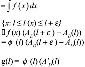 

and hence (2).

Evidently, a sufficient condition that the mode of f(x) coincides with the minimizer of l(x) is that φ (x) be monotone decreasing and assuming differentiability, then

(5) 

The positivity of φ (l(x)) = f(x)) requires that A'(l)≥0. Next taking the logarithmic derivative of (4) yields

(6) 

and therefore

(7)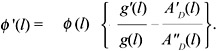 

Since φ (l) =f(x) ≥ 0, we therefore have proven

Theorem 3: The mode of the f(x) density (expert estimates) identifies the minimum point of l(x) if

(8)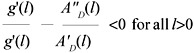 

Condition (8) shows the required relationship between the loss function, l(x), and the expertise density, g(l) in order that the mode of f(x) identifies the most accurate estimate. The next two examples illustrate its use.

Example 1: Suppose k_l and k₂ > 0 and let

(9)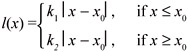 

Let g(l) be an arbitrary differentiable monotone decreasing density on l ≥ 0. (For example, g(l) = μe^-μ1, μ > 0.) Here A(l) = (1/k₁ + l/k₂) with A "(l) = 0. Hence (9) holds since g'(l)<0.

Example 2: Let l(x) = k(x - x₀)² and suppose g(l) = μe^-μ1, μ > 0. Hence A(l) = 2(l/k)^1/2, with A'(l) = (l/k)^1/2(1/k) = k^1/2l^-1/2 and A"(l) = -1/2k^-1/2l^-3/2. Thus

(10)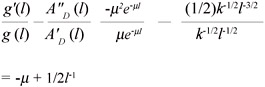 

for any μ > 0 there exist values of l such that (10) will be positive. Therefore the ideal point cannot be identified by the mode of the expert estimates. In fact, the density, f(x), for this case can be derived using (2) as f(x) = µ|x| exp{-μx²} which is easily seen to be bimodal.

To summarize, the mode of expert estimates will tend to identify the most accurate estimate under a wide variety of loss functions, l(x) provided that

1. Estimates of equal l(x) value, l, are uniformly distributed on the set {x: l(x)= l}. In the case of convex l(x) functions, there are two such values, each of equal likelihood.

2. Condition (8) holds.

These results suggest that, in general, the mode of individual forecasts should be expected to be an effective and simple maximum likelihood method for forecast combination. It has the potential advantage over the simple average forecast in that the l(x) function may be skewed from trial to trial, even though the performance density may be essentially constant. In "Individual and Combination Forecasts" and "Bayesian Approach," a particular mode estimator, the classical Pearson mode estimate, is obtained in a Markov chain Monte Carlo framework. The results are then applied and compared to five individual and other combination methods.

---