An Example from Software Design and Development

As our first example of a software design application of Taguchi Methods, we will consider a software program improvement project for the Indian government. It was created by B. Kanchana and published as his doctoral dissertation at the Indian Institute of Science at Bangalore.^[5] Most software design projects start with an existing program rather than a blank sheet of paper (or a blank programming screen these days), so our example exhibits little loss of generality as a typical software design project. This Indian Defense Ministry project was to redesign the man-machine interface display (MMID) subsystem of the Airborne Surveillance Platform (ASP) system, which was programmed in the C language. The quality goal was to reduce the number of errors per module in the system shown in hierarchical form in Figure 17.4. This subsystem employs a user interface device to provide access protocol, equipment control, and operations oversight, and it displays the air surveillance situation on a color display.

Figure 17.4. Architecture of the MMID Subsystem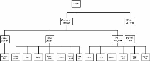

Each engagement of the system lasts five or six hours and involves thousands of data words scanned every few seconds. Figure 17.5 shows part of the cause-and-effect diagram for typical design faults in the project's requirements, specification, and design phases. The two major modules of MMID, Receive_plot_data() and Command_proc_task(), are shown in Figure 17.6. Receive_plot_data() displays plot data in screen coordinates, and Command_proc_task() handles azimuth display, range ring display, and maximum range detection. The first factor is the number of requirements per module. The second is the cyclomatic complexity of each module. The third is coupling modes between modules, data coupling (call by value), stamp coupling (call by name), control coupling (method invocation), common data coupling (global data reference), and content coupling (remote method invocation), in increasing complexity. These parameters or control factors are listed together with their possible levels in Table 17.4.

Figure 17.5. A Typical Cause-and-Effect Diagram for Design Faults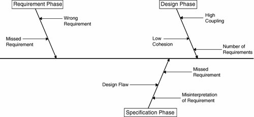

Figure 17.6. Major Modules of the MMID Subsystem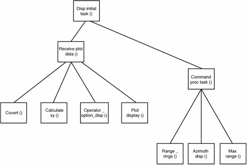

Table 17.4. Control Factors and Their Levels

Label	Control Factor Name	Level 1	Level 2	Level 3
A	Number of requirements per module	1	2	>2
B	Cyclomatic complexity	<5	510	>10
C	Coupling	Data, stamp, and control	Common, content

A factorial experiment to consider all possible factor level combinations of these would require 18 experiments because A is at three levels, B is at three levels, and C is at two levels, and 3 x 3 x 2 = 18. Taguchi has tabulated a series of orthogonal arrays for use in such experiments. L₉ (for a nine-row Latin square) is the appropriate array for this data set, as shown in Table 17.5.

Table 17.5. Taguchi's L₉ Orthogonal Array

Experiment	A	B	C
1	1	1	1
2	1	2	2
3	1	3	3 = 2
4	2	1	2
5	2	2	3 = 2
6	2	3	1
7	3	1	3 = 2
8	3	2	1
9	3	3	2

For each experiment, a number of modules are tested for errors, as shown in Table 17.6. Kanchana computed the SNR as

Table 17.6. Experimental Results

Experiment	Module Name	Errors	Average Per Module	SNR
1	Azimuth() Calc_xy_pos()	2 1	1.5	3.98
2	Curr_opt_option() Sector_proc() Hndl_async_calls()	1 2 1	1.333	3.01
3	Glb3_var() Fan_out() Fan_in() Tx_sec_menu_proc() Security_ clearance()	2 2 2 3 3	2.0	6.02
4	Track_ret_opt() Sys_data_in_out()	2 1	1.5	3.98
5	Prev_curr_scan_disp() Date_time_input()	1 3	2.0	6.98
6	Elapsed_time() Mod1_nam()	1 3	2.0	6.98
7	Receive_data() Current_status()	2 1	1.5	3.98
8	Peridoc_hlth_task() Handle_dbit_PRF() Get_dbit_PRF_ack()	1 2 2	1.66	4.77
9	Overlay() Set_mission_time() Receive_plot_data()	1 6 31	3.33	11.89

S/N(θ) = -10 log₁₀ [Σ(y_i²/n)], i = 1, n

in which θ= (θ₁, θ₂,..., θ_k) is the vector of control parameters, and y = (y₁, y₂,...,y_k) is the vector of performance statistics. You repeat each observation n times at each selected combination of design parameter sets in the orthogonal array. The best setting of the design parameters is the one that maximizes the SNRin this case, the type 2 experiment. In other words, it's the case in which cyclomatic complexity is maintained at level 2, coupling is kept at level 2, and the number of requirements per module is kept at level 1.

To verify these results, Kanchana examined the error-prone module Set_mission_time() and discovered that it had a cyclomatic complexity of 18, two requirements per module, and employed common coupling. To improve MMID quality, this module was split into six smaller modules. After coding, they were tested to discover only one error in one of them rather than the six in the first version. Likewise, Security_clearance() was examined to discover a cyclomatic complexity of 12 and common coupling but only level 1 requirements. It was split into five modules, none of which showed any errors upon testing. The conclusion in Kanchana's dissertation and in a later presentation^[6] was that the optimal design parameters for MMID are one requirement per module, coupling by data passing whenever possible, and limiting cyclomatic complexity to less than 10.