Orthogonal Matrices for Taguchi Parameter Design Experiments

This section presents more technical details for the use of the reduced factorial or orthogonal matrix method so central to Taguchi Methods. The full nomenclature for an orthogonal array is L_a(b^c), in which L stands for Latin square, a is the number of test trials, b is the number of levels for each column, and c is the number of columns in the array. An orthogonal matrix is a generalized Latin square. For example, the L₄(2³) orthogonal array is shown in Table 17.7.

Table 17.7. An L₄(2³) Orthogonal Array

Number	1	2	3
1	1	1	1
2	1	2	2
3	2	1	2
4	2	2	1

Appendix B of the Robust Engineering Workshop Manual from the American Supplier Institute gives schemata for orthogonal arrays up to L₅₄(3³⁵).^[7]

We want to use such matrices to represent the design values and trade-offs over which the design engineer has a choice, as well as the noise factors that may cause the product to deviate from the target (and thus quality) when used in its operational environment. This is the second stage in a Taguchi robust engineering design process. The first is designing to meet user-expressed functional requirements. The third stage is tolerance design, in which the engineer must tighten tolerances on components that cannot be made adequately robust by parameter design. Successful parameter design is the essence of Taguchi Methods. We start with a product that is designed to meet the user's requirements, but now we want to ensure that it will do so all the time, and thus exhibit robustness in the face of adverse real-world environmental and usage factors. The great advantage of parameter design is that it adds robustness without adding cost; in fact, it reduces costs by eliminating unnecessary components, and of course future warranty claims and later rework. Tolerance design is employed only when parameter design does not meet all the implicit robustness requirements and almost always adds cost to the actual product, even though it does contribute positively to the quality loss function itself.

Figure 17.7, adapted from a popular and readily available statistical handbook,^[8] presents a small L₉ orthogonal matrix that is large enough to support a more detailed discussion of the parameter design or optimization process for a product, whether hardware or software. The columns of the design parameter matrix represent the design parameters, and its rows represent different combinations of test settings. The noise factor matrix specifies the test levels for the noise factors. Its columns identify the noise factors, and its rows represent the different combinations of noise factors applied simultaneously. In reality, the engineer has no control over either the levels or combinations of noise factors. But in the parameter design experiment, he can try different levels and combinations in such a way as to stress his design and optimize its robustness against such uncontrollable factors. Each test run of the design parameter matrix is crossed with every row of the noise factor matrix. In this way, virtual product performance mimics future real product performance variation at given design parameter settings. The result of the statistical experiment is a performance statistic that estimates or predicts the effect of the noise factors on expected performance for the controllable parameter combinations. A preferred combination of design parameters is identified by an objective function such as the SNR. The prediction then is verified by a confirmation experiment, and several iterations may be required to minimize the object function. Parameter design experimental data may be gathered by actual physical experiments or by simulation trials using a performance model.

Figure 17.7. Taguchi Parameter Design Schema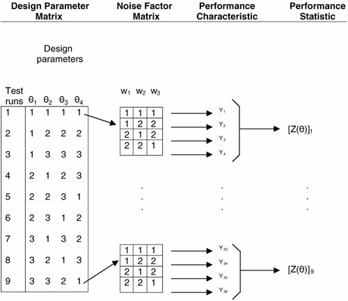

A performance statistic estimates the effect of noise factors on a performance characteristic. If θ= (θ₁, θ₂...θ_k) is the vector of design parameters and w = (w₁,w₂...w_t) is the vector of noise factors, and the performance factor Y is a function of θ and w, Y = f (θ, w). We can further define the following functions of θ:^[9]

Mean	η (θ) = E[Y]
Variance	σ2 (θ) = E [{Y η (θ)}2]
Coefficient of variation	CV (θ) = σ (θ)/ η(θ)
Mean squared error	MSE(θ) = E[(Y τ)2]
Bias of distribution of Y	B(θ) = η(θ) τ

in which τ is the target value. Three possible optimization situations occur, depending on the target value. If the target value is 0, if Y has a nonnegative distribution, and if the loss function L(Y) increases as Y increases, the expected loss is proportional to

MSE (θ) = E[(Y 0)²] = E[Y²]

In this case, Taguchi recommends the performance measure 10 log MSE(θ). If the target value is infinity, if the distribution of Y is positive, and if the loss function decreases as Y decreases, Taguchi recommends using 1/Y as the performance characteristic so that the target value of 1/Y becomes 0. On the other hand, if a specific target value τ = τ₀ is desired, and the loss function increases symmetrically and Y deviates from the desired target value τ₀ in either direction, the loss function L(Y) is proportional to MSE(θ) = E[(Y τ₀)²], so that MSE(θ) = σ²(θ) + [B(θ)]² and σ(θ) = CV(θ) η(θ).