5.5 Adaptive Space-Time Multiuser Detection in Synchronous CDMA

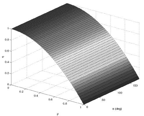
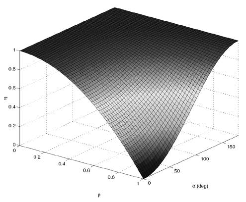
Generally speaking, space-time processing involves the exploitation of spatial diversity using multiple transmit and/or receive antennas and, perhaps, some form of coding. In previous sections we have focused on systems that employ one transmit antenna and multiple receive antennas. Recently, however, much of the work in this area has focused on transmit diversity schemes that use multiple transmit antennas. They include delay schemes [444, 572, 573] in which copies of the same symbol are transmitted through multiple antennas at different times, the space-time trellis coding algorithm in [477], and the simple space-time block coding (STBC) scheme developed in [12], which has been adopted in third-generation (3G) wideband CDMA (WCDMA) standards [294, 479]. A generalization of this simple space-time block coding concept is developed in [475, 476]. It has been shown that these techniques can significantly increase capacity [122, 478].

In this section we discuss adaptive receiver structures for synchronous CDMA systems with multiple transmit antennas and multiple receive antennas. Specifically, we focus on three configurations: (1) one transmit antenna, two receive antennas; (2) two transmit antennas, one receive antenna; and (3) two transmit antennas, two receive antennas. It is assumed that the orthogonal space-time block code [12] is employed in systems with two transmit antennas. For each of these configurations, we discuss two possible linear receiver structures and compare their performance in terms of diversity gain and signal separation capability. We also describe blind adaptive receiver structures for such multiple-antenna CDMA systems. The methods discussed in this section are generalized in the next section to mutipath CDMA systems. The materials discussed in this and the following sections first appeared in [415].

5.5.1 One Transmit Antenna, Two Receive Antennas

Consider the following discrete-time K - user synchronous CDMA channel with one transmit antenna and two receive antennas. The received baseband signal at the p th antenna can be modeled as

Equation 5.95

where s _k is the N -vector of the discrete-time signature waveform of the k th user with unit norm (i.e., s _k = 1), b _k {+1, “1} is the data bit of the k th user, g _p,k is the complex channel response of the p th receive antenna element to the k th user's signal, and n _p ~ N _c ( , s ² I _N ) is the ambient noise vector at antenna p . It is assumed that n ₁ and n ₂ are independent.

Linear Diversity Multiuser Detector

Denote

Suppose that user 1 is the user of interest. We first consider the linear diversity multiuser detection scheme, which first applies a linear multiuser detector to the received signal r _p in (5.95) at each antenna p = 1, 2, and then combines the outputs of these linear detectors to make a decision. For example, a linear decorrelating detector for user 1 based on the signal in (5.95) is simply

Equation 5.96

where e ₁ denotes the first unit vector in . This detector is applied to the received signal at each antenna p = 1, 2, to obtain z = [ z ₁ z ₂ ] ^T , where

Equation 5.97

with

Equation 5.98

where w ₁ ² = [ R ^“1 ] _1,1 . Denote

Equation 5.99

and . Since the noise vectors from different antennas are independent, we can write

Equation 5.100

with

Equation 5.101

The maximum- likelihood (ML) decision rule for b ₁ based on z in (5.100) is then

Equation 5.102

Let be the total received desired user's signal energy. The decision statistic in (5.102) can be expressed as

Equation 5.103

with

Equation 5.104

The probability of detection error is computed as

Equation 5.105

Linear Space-Time Multiuser Detector

Denote

Then, by augmenting the received signals at two antennas, (5.95) can be written as

Equation 5.106

with . A linear space-time multiuser detector operates on the augmented received signal directly. For example, the linear decorrelating detector for user 1 in this case is given by

Equation 5.107

This detector is applied to the augmented received signal to obtain

Equation 5.108

with

Equation 5.109

where . Denote

Equation 5.110

An expression for can be found as follows . Note that

Equation 5.111

Equation 5.112

where (5.111) and (5.112) follow, respectively, from the following two matrix identities:

Equation 5.113

Equation 5.114

Hence

Equation 5.115

where ° denotes the Schur matrix product (i.e., elementwise product).

The ML decision rule for b ₁ based on in (5.108) is then

Equation 5.116

The probability of detection error is computed as

Equation 5.117

Performance Comparison

From the discussion above it is seen that the linear space-time multiuser detector exploits the signal structure in both the time domain (i.e., induced by the signature waveform s _k ) and the spatial domain (i.e., induced by the channel response g _k ) for interference rejection; whereas for the linear diversity multiuser detector, interference rejection is performed only in the time domain, and the spatial domain is used only for diversity combining. The next result, which first appeared in [324], shows that the linear space-time multiuser detector always outperforms the linear diversity multiuser detector.

Proposition 5.6: Let ( e ) given by (5.105) and ( e ) given by (5.117) be, respectively, the probability of detection error of the linear diversity detector and the linear space-time detector. Then

Proof: By (5.105) and (5.117) it suffices to show that

We make use of the following facts. Denote by A _i,j the submatrix of A obtained by striking out the i th row and the j th column. Then it is known that

Equation 5.118

It is also known that

Equation 5.119

Assuming that and , and using the two results above, we have

Equation 5.120

Equation 5.121

Equation 5.122

where (5.120) follows from the fact that and ; (5.121) follows from the matrix identity

Equation 5.123

and (5.122) follows from

Equation 5.124

Hence we have

Equation 5.125

We next consider a simple example to demonstrate the performance difference between the two receivers discussed above. Consider a two-user system with

where r is the correlation of the signature waveforms of the two users and q ₁ and q ₂ are the directions of arrival of the two users' signals. Define . Then we have E ₁ = E ₂ = 1 and

Equation 5.126

Equation 5.127

Equation 5.128

Equation 5.129

These expressions are plotted in Fig. 5.12. It is seen that while the multiuser space-time receiver can exploit both the temporal signal separation (along the r -axis) and the spatial signal separation (along the a -axis), the multiuser diversity receiver can exploit only the temporal signal separation. For example, for large r , the performance of the multiuser diversity receiver is poor, no matter what value a takes; but the performance of the multiuser space-time receiver can be quite good as long as a is large.

Figure 5.12. Performance comparison between a multiuser diversity receiver (top) and multiuser space-time receiver (bottom).

5.5.2 Two Transmit Antennas, One Receive Antenna

When two antennas are employed at the transmitter, we must first specify how the information bits are transmitted across the two antennas. Here we adopt the well-known orthogonal space-time block coding scheme [12, 475]. Specifically, for user k , two information symbols, b _{k ,1} and b _{k ,2} , are transmitted over two symbol intervals. At the first time interval, the symbol pair ( b _{k ,1} , b _{k ,2} ) is transmitted across the two transmit antennas; and at the second time interval, the symbol pair ( “ b _{k ,2} , b _{k ,1} ) is transmitted. The received signals corresponding to these two time intervals are given by

Equation 5.130

Equation 5.131

where g _{1, k} ( g _{2, k} ,) is the complex channel response between the first (second) transmit antenna and the receive antenna; n ₁ and n ₂ are independent received N _c ( 0, I _N ) noise vectors at the two time intervals.

Linear Diversity Multiuser Detector

We first consider the linear diversity multiuser detection scheme, which first applies the linear multiuser detector w ₁ in (5.96) to the received signals r ₁ and r ₂ during the two time intervals, and then performs a space-time decoding. Specifically, denote

Equation 5.132

Equation 5.133

with

Equation 5.134

where w ₁ ² = [ R ^“1 ] _1,1 .

Denote

It is easily seen that . Then (5.132) “(5.134) can be written as

Equation 5.135

with

Equation 5.136

As before, denote . Note that

Equation 5.137

The ML decision rule for b _1,1 and b _2,1 based on z in (5.135) is then given by

Equation 5.138

Using (5.135), it is easily seen that the decision statistic in (5.138) is distributed according to

Equation 5.139

Equation 5.140

Hence the probability of error is given by

Equation 5.141

This is the same expression as (5.117) for the linear diversity receiver with one transmit antenna and two receive antennas.

Linear Space-Time Multiuser Detector

Denote and . Then (5.130) and (5.131) can be written as

Equation 5.142

On denoting

the decorrelating detector for detecting the bit b _1,1 based on in (5.142) is given by

Equation 5.143

where is the first unit vector in . We have the following result.

Proposition 5.7: The decorrelating detector in (5.143) is given by

Equation 5.144

where w ₁ is given by (5.96).

Proof: We need to verify that

Equation 5.145

We have

Equation 5.146

Equation 5.147

Equation 5.148

Equation 5.149

This verifies (5.145), so that (5.144) is indeed the decorrelating detector given by (5.143).

Thus the output of the linear space-time detector in this case is given by

Equation 5.150

with

Equation 5.151

where using (5.99) and (5.144), we have

Equation 5.152

Therefore, the probability of detection error is given by

Equation 5.153

On comparing (5.141) with (5.153) we see that for the case of two transmit antennas and one receive antenna, the linear diversity receiver and the linear space-time receiver have the same performance. Hence the multiple transmit antennas with space-time block coding provide only diversity gain and no signal separation capability.

5.5.3 Two Transmit and Two Receive Antennas

We combine the results from the two preceding sections to investigate an environment in which we use two transmit antennas and two receive antennas. We adopt the space-time block coding scheme used in the preceding section. The received signals at antenna 1 during the two symbol intervals are

Equation 5.154

Equation 5.155

and the corresponding signals received at antenna 2 are

Equation 5.156

Equation 5.157

where is the complex channel response between transmit antenna i and receive antenna j for user k . The noise vectors , and are independent and identically distributed with distribution N _c ( , s ² I _N ).

Linear Diversity Multiuser Detector

As before, we first consider the linear diversity multiuser detection scheme for user 1, which applies the linear multiuser detector w ₁ in (5.96) to each of the four received signals , and and then performs a space-time decoding. Specifically, denote the filter outputs as

Equation 5.158

Equation 5.159

Equation 5.160

Equation 5.161

with

Equation 5.162

where, as before, .

We define the following quantities :

Then (5.158) “(5.162) can be written as

Equation 5.163

with

Equation 5.164

It is readily verified that

Equation 5.165

with

Equation 5.166

To form the ML decision statistic, we premultiply z by G ₁ and obtain

Equation 5.167

with

Equation 5.168

The corresponding bit estimates are given by

Equation 5.169

The bit error probability is then given by

Equation 5.170

Linear Space-Time Multiuser Detector

We denote

Then (5.154) “(5.157) may be written as

Equation 5.171

Equation 5.172

where

Since and (5.171) has the same form as (5.142), it is easy to show that the decorrelating detector for detecting the bit b _1,1 based on is given by

Equation 5.173

Hence the output of the linear space-time detector in this case is given by

Equation 5.174

with

Equation 5.175

where

Equation 5.176

Therefore, the probability of detection error is given by

Equation 5.177

Comparing (5.177) with (5.170), it is seen that when two transmit antennas and two receive antennas are employed and the signals are transmitted in the form of a space-time block code, the linear diversity receiver and the linear space-time receiver have identical performance.

Remarks

We have seen that the performance of space-time multiuser detection (STMUD) and linear diversity multiuser detection (LDMUD) are similar for two transmit/one receive and two transmit/two receive antenna configurations. What, then, are the benefits of the space-time detection technique? They are as follows:

1. Although LDMUD and STMUD perform similarly for the 2 x 1 and 2 x 2 cases, the performance of STMUD is superior for configurations with one transmit antenna and P 2 receive antennas.

2. User capacity for CDMA systems is limited by correlations among composite signature waveforms. This multiple-access interference will tend to decrease as the dimension of the vector space in which the signature waveforms reside increases . The signature waveforms for linear diversity detection are of length N (i.e., they reside in ). Since the received signals are stacked for space-time detection, these signature waveforms reside in for two transmit and one receive antennas or for two transmit and two receive antennas. As a result, the space-time structure can support more users than linear diversity detection for a given performance threshold.

3. For adaptive configurations (Section 5.5.4 and Section 5.6.2), LDMUD requires four independent subspace trackers operating simultaneously since the receiver performs detection on each of the four received signals, and each has a different signal subspace. The space-time structure requires only one subspace tracker.

5.5.4 Blind Adaptive Implementations

We next develop both batch and sequential blind adaptive implementations of the linear space-time receiver. These implementations are blind in the sense that they require only knowledge of the signature waveform of the user of interest. Instead of the decorrelating detector used in previous sections, we will use a linear MMSE detector for the adaptive implementations because the MMSE detector is more suitable for adaptation and its performance is comparable to that of the decorrelating detector. We consider only the environment in which we have two transmit antennas and two receive antennas. The other cases can be derived in a similar manner. Note that inherent to any blind receiver in multiple transmit antenna systems is an ambiguity issue. That is, if the same spreading waveform is used for a user at both transmit antennas, the blind receiver cannot distinguish which bit is from which antenna. To resolve such an ambiguity, here we use two different spreading waveforms for each user (i.e., s _j,k , j {1, 2} is the spreading code for user k for the transmission of bit b _{j, k} ).

There are two bits, b _{1, k} [ i ] and b _{2, k} [ i ], associated with each user at each time slot i , and the difference in time between slots is 2 T , where T is the symbol interval. The received signal at antenna 1 during the two symbol periods for time slot i is

Equation 5.178

Equation 5.179

and the corresponding signals received at antenna 2 are

Equation 5.180

Equation 5.181

We stack these received signal vectors and denote

Then we may write

Equation 5.182

where

The autocorrelation matrix of the stacked signal [ i ], C , and its eigendecomposition are given by

Equation 5.183

Equation 5.184

where L _s = diag { l ₁ , l ₂ , . . . , l _{2 K} } contains the largest (2 K ) eigenvalues of C , the columns of U _s are the corresponding eigenvectors, and the columns of U _n are the 4 N “ 2 K eigenvectors corresponding to the smallest eigenvalue s ² .

The blind linear MMSE detector for detecting [ b [ i ]] ₁ = b _1,1 [ i ] is given by the solution to the optimization problem

Equation 5.185

From Chapter 2, a scaled version of the solution can be written in terms of the signal subspace components as

Equation 5.186

and the decision is made according to

Equation 5.187

and

Equation 5.188

or

Equation 5.189

Before we address specific batch and sequential adaptive algorithms, we note that these algorithms can also be implemented using linear group -blind multiuser detectors instead of blind MMSE detectors. This would be appropriate, for example, in uplink environments in which the base station has knowledge of the signature waveforms of all of the users in the cell, but not those of users outside the cell . Specifically, we may rewrite (5.182) as

Equation 5.190

where we have separated the users into two groups. The composite signature sequences of the known users are the columns of . The unknown users' composite sequences are the columns of . Then, from Chapter 3, the group-blind linear hybrid detector for bit b _1,1 [ i ] is given by

Equation 5.191

This detector offers a significant performance improvement over (5.186) for environments in which the signature sequences of some of the interfering users are known.

Batch Blind Linear Space-Time Multiuser Detection

To obtain an estimate of g ₁ , we make use of the orthogonality between the signal and noise subspaces [i.e., the fact that . In particular, we have

Equation 5.192

Equation 5.193

In (5.193), specifies g ₁ up to an arbitrary complex scale factor a (i.e., ). The following is a summary of a batch blind space-time multiuser detection algorithm for the two transmit antenna/two receive antenna configuration.

Algorithm 5.4: [Batch blind linear space-time multiuser detector ”synchronous CDMA, two transmit antennas, and two receive antennas]

• Estimate the signal subspace:

  Equation 5.194

  

  
  

  Equation 5.195

  

  
  

• Estimate the channels:

  Equation 5.196

  

  
  

  Equation 5.197

  

  
  

  Equation 5.198

  

  
  

  Equation 5.199

  

  
  

• Form the detectors:

  Equation 5.200

  

  
  

  Equation 5.201

  

  
  

• Perform differential detection:

  Equation 5.202

  

  
  

  Equation 5.203

  

  
  

  Equation 5.204

  

  
  

  Equation 5.205

  

  
  

A batch group-blind space-time multiuser detector algorithm can be implemented with simple modifications to (5.200) and (5.201).

Adaptive Blind Linear Space-Time Multiuser Detection

To form a sequential blind adaptive receiver, we need adaptive algorithms for sequentially estimating the channel and the signal subspace components U _s and L _s . First, we address sequential adaptive channel estimation. Denote by z [ i ] the projection of the stacked signal [ i ] onto the noise subspace:

Equation 5.206

Equation 5.207

Since z [ i ] lies in the noise subspace, it is orthogonal to any signal in the signal subspace, and in particular, it is orthogonal to ( ). Hence g ₁ is the solution to the following constrained optimization problem:

Equation 5.208

To obtain a sequential algorithm to solve the optimization problem above, we write it in the following (trivial) state space form:

The standard Kalman filter can then be applied to the system above as follows. Denote . We have

Equation 5.209

Equation 5.210

Equation 5.211

Once we have obtained channel estimates at time slot i , we can combine them with estimates of the signal subspace components to form the detector in (5.186). Since we are stacking received signal vectors, and subspace tracking complexity increases at least linearly with signal subspace dimension, it is imperative that we choose an algorithm with minimal complexity. The best existing low-complexity algorithm for this purpose appears to be the NAHJ subspace tracking algorithm discussed in Section 2.6.3. This algorithm has the lowest complexity of any algorithm used for similar purposes and has performed well when used for signal subspace tracking in multipath fading environments. Since the size of U _s is 4 N x 2 K , the complexity is 40 · 4 N · 2 K + 3 · 4 N + 7.5(2 K ) ² + 7 · 2 K floating point operations per iteration.

Algorithm 5.5: [Blind adaptive linear space-time multiuser detector ”synchronous CDMA, two transmit antennas, and two receive antennas]

• Using a suitable signal subspace tracking algorithm (e.g., NAHJ), update the signal subspace components U _s [ i ] and L _s [ i ] at each time slot i.

• Track the channel g ₁ [ i ] and according to the following:

  Equation 5.212

  

  
  

  Equation 5.213

  

  
  

  Equation 5.214

  

  
  

  Equation 5.215

  

  
  

  Equation 5.216

  

  
  

  Equation 5.217

  

  
  

  Equation 5.218

  

  
  

  Equation 5.219

  

  
  

  Equation 5.220

  

  
  

• Form the detectors:

  Equation 5.221

  

  
  

  Equation 5.222

  

  
  

• Perform differential detection:

Equation 5.223

Equation 5.224

Equation 5.225

Equation 5.226

A group-blind sequential adaptive space-time multiuser detector can be implemented similarly. The adaptive receiver structure is illustrated in Fig. 5.13.

Figure 5.13. Adaptive receiver structure for linear space-time multiuser detectors.