2.8 Appendix

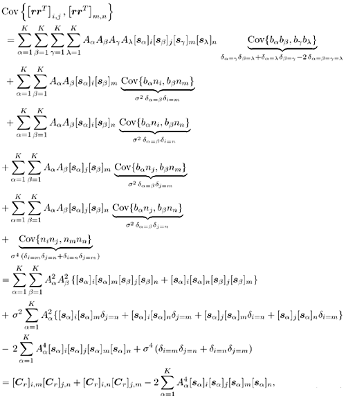
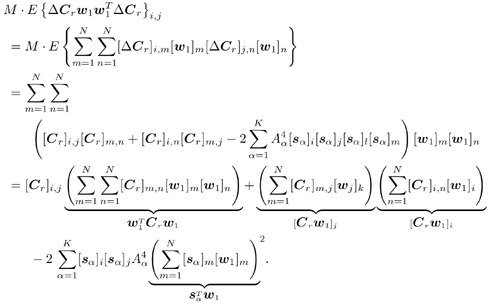
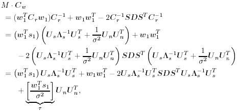
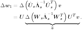
2.8.1 Derivations for Section 2.3.3

Derivation of Equation (2.61)

Recall that the RLS algorithm for updating the blind linear MMSE algorithm is as follows :

Equation 2.247

Equation 2.248

Equation 2.249

Equation 2.250

Equation 2.251

We first derive an explicit recursive relationship between m ₁ [ i ] and m ₁ [ i -1]. Define

Equation 2.252

Premultiplying both sides of (2.249) by , we get

Equation 2.253

From (2.253), we obtain

Equation 2.254

where

Equation 2.255

Substituting (2.249) and (2.254) into (2.250), we get

Equation 2.256

where

Equation 2.257

is the a priori least-squares estimate at time i . It is shown below that

Equation 2.258

Equation 2.259

Substituting (2.248) and (2.258) into (2.256), we get

Equation 2.260

Therefore, by (2.260) we have

Equation 2.261

where v [ i ] is defined in (2.56). Therefore, from (2.261) we get

Equation 2.262

Finally, we derive (2.258) and (2.259). Postmultipling both sides of (2.251) by r [ i ], we get

Equation 2.263

On the other hand, (2.247) can be rewritten as

Equation 2.264

Equation (2.258) is obtained by comparing (2.263) and (2.264). Multiplying both sides of (2.254) by k [ i ], we get

Equation 2.265

Equation (2.255) can be rewritten as

Equation 2.266

Equation (2.259) is obtained comparing (2.265) and (2.266).

Derivation of Equations (2.62) “(2.69)

Suppose that an application of the rotation matrix Q [ i ] yields the following form:

Equation 2.267

Then because of the orthogonality property of Q [ i ] (i.e., ), taking the outer products of each side of (2.267) with their respective Hermitians, we get the following identities:

Equation 2.268

Equation 2.269

Equation 2.270

Associating A ₁ with the first N columns of the partitioned matrix on the left-hand side of (2.62), and B ₁ with the first N columns of the partitioned matrix on the right-hand side of (2.62), then (2.268), (2.269), and (2.270) yield

Equation 2.271

Equation 2.272

Equation 2.273

Equation 2.274

Equation 2.275

Equation 2.276

A comparison of (2.271) “(2.273) with (2.54) “(2.56) shows that C [ i ], u [ i ], and v [ i ] in (2.62) are the correct updated quantities at time n . Moreover, (2.67) follows from (2.274) and (2.57), (2.68) follows from (2.275) and (2.59), and (2.69) follows from (2.276) and (2.262).

2.8.2 Proofs for Section 2.4.4

Proof of Lemma 2.3

Denote

Note that the eigendecomposition of H is given by

Equation 2.277

Then the Moore “Penrose generalized inverse [189] of matrix H is given by

Equation 2.278

On the other hand, the Moore “Penrose generalized inverse H of a matrix H is the unique matrix that satisfies [189] (a) HH and H H are symmetric; (b) HH H = H ; and (c) H HH = H . Next we show that G = H by verifying these three conditions. We first verify condition (a). Using (2.106), we have

Equation 2.279

where the second equality follows from the facts that W ^T W = I _N and S ^T S ^T = V ^T V = VV ^T = I _K . Since the N x N diagonal matrix S S = diag ( I _K , ), it follows from (2.279) that HG is symmetric. Similarly, GH is also symmetric. Next we verify condition (b).

Equation 2.280

where in the second equality, the following facts are used: W ^T W = I _N , S ^T S ^T = I _K , and V ^T V = VV ^T = I _K ; the third equality follows from the fact that S S S = S . Condition (c) can be similarly verified (i.e., GHC = G ). Therefore, we have

Equation 2.281

Now (2.107) follows immediately from (2.281) and the fact that U ^T U = UU ^T = I _N .

2.8.3 Proofs for Section 2.5.2

Some Useful Lemmas

We first list some lemmas that will be used in proving the results in Section 2.5.2. A random matrix is said to be Gaussian distributed if the joint distribution of all its elements is Gaussian. First we have the following vector form of the central limit theorem.

Lemma 2.4: (Theorem 1.9.1B in [443]) Let { x _i } be i.i.d. random vectors with mean m and covariance matrix S . Then

Next we establish that the sample autocorrelation matrix given by (2.122) is asymptotically Gaussian distributed as the sample size M .

Lemma 2.5 Denote

Equation 2.282

Equation 2.283

Equation 2.284

Then converges in probability toward a Gaussian matrix with mean and an N ² x N ² covariance matrix whose elements are specified by

Equation 2.285

Proof: Since given by (2.285) has , and it is a sum of i.i.d. terms ( r [ i ] r [ i ] ^T ), by Lemma 2.4, it is asymptotically Gaussian, with an N ² x N ² covariance matrix whose elements are given by the covariance of the zero-mean random matrix ( r [ i ] r [ i ] ^T ). To calculate this covariance, note that (for notational convenience, in what follows we drop the time index i )

Equation 2.286

We have

Equation 2.287

where the last equality follows from the fact that

Equation 2.288

Note that the last term of (2.285) is due to the nonnormality of the received signal r [ i ]. If the signal had been Gaussian, the result would have been the first two terms of (2.285) only (compare this result with Theorem 3.4.4 in [18]). Using a different modulation scheme (other than BPSK) will result in a different form for the last term in (2.285).

In what follows we make frequent use of the differential of a matrix function (cf. [421], Chap. 14). Consider a function . Recall that the differential of f at a point x is a linear function such that

Equation 2.289

If the differential exists, it is given by L _f ( x ; x ) = T ( x ) x , where . Let y = f ( x ) and consider its differential at x . Denote . Hence for fixed x , D y is a function of D x ; and for fixed x , if x is random, so is D y . We have the following lemma regarding the asymptotic distribution of a function of a sequence of asymptotically Gaussian vectors.

Lemma 2.6: (Theorem 3.3A in [443]) Suppose that is asymptotically Gaussian; that is ,

Let be a function . Denote y ( M )= f [ x ( M )]. Suppose that f has a nonzero differential L _f ( x ; x ) = T ( x ) x at x . Denote and D y ( M ) = T ( x ) D x ( M ). Then

Equation 2.290

where

Equation 2.291

Equation 2.292

To calculate C _y we can use either (2.291) or (2.292). When dealing with functions of matrices, however, it is usually easier to use (2.292). In what follows we make use of the following identities of matrix differentials:

Equation 2.293

Equation 2.294

Equation 2.295

Finally, we have the following lemma regarding the differentials of the eigencomponents of a symmetric matrix. It is a generalization of Theorem 13.5.1 in [18]. Its proof can be found in [197].

Lemma 2.7: Let the N x N symmetric matrix C have an eigendecomposition , where the eigenvalues satisfy . Let D C be a symmetric variation of C and denote . Let T be a unitary transformation of C as

Equation 2.296

Denote the eigendecomposition of T as

Equation 2.297

(Note that if C = C , then W = I _N and L = L .) The differential of L at L , and the differential of W at I _N , as a function of , are given, respectively, by

Equation 2.298

Equation 2.299

Proof of Theorem 2.1

DMI Blind Detector Consider the function . The differential of at C _r is given by

Equation 2.300

where . Then according to Lemma 2.6, is asymptotically Gaussian as M , with zero mean and covariance matrix given by (2.292) ^[4]

^[4] We do not need the limit here, since the covariance matrix of is independent of M .

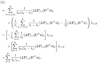
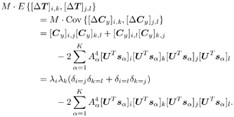
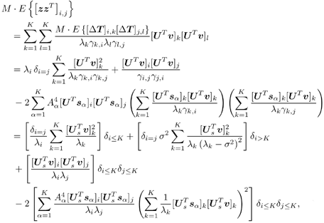
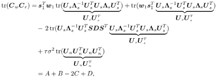
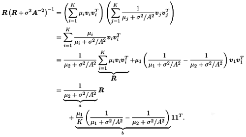
Equation 2.301

Now, by Lemma 2.5, we have

Equation 2.302

Writing (2.302) in a matrix form, we have

Equation 2.303

with

The eigendecomposition of C _r is

Equation 2.304

Substituting (2.303) and (2.304) into (2.301), we get

where the last equality follows from the fact that .

Subspace Blind Detector We will prove the following more general proposition, which will be used in later proofs. The part of Theorem 2.1 for the subspace blind detector follows with v = s ₁ .

Proposition 2.6: Let be the weight vector of a detector , and let be the weight vector of the corresponding estimated detector. Then

with

Equation 2.305

where

Equation 2.306

Equation 2.307

Proof: Consider the function . By Lemma 2.6, is asymptotically Gaussian as M , with zero mean and covariance matrix given by where D w ₁ is the differential of at ( U _s , L _s ). Denote U = [ U _s U _n ]. Define

Equation 2.308

Since T is a unitary transformation of , its eigenvalues are the same as those of . Hence its eigendecomposition can be written as

Equation 2.309

where are eigenvectors of T . From (2.308) and (2.309), we have

Equation 2.310

Thus we have

Equation 2.311

The differential in (2.311) at ( I _N , L ) is given by

Equation 2.312

where E _s is composed of the first K columns of I _N . Using Lemma 2.7, after some manipulations, we have

Equation 2.313

with

Equation 2.314

where we have used the fact that D T is symmetric (i.e., [ D T ] _i,j = [ D T ] _j,i ). Denote

Equation 2.315

Then C _y = U ^T C _r U = L . Moreover, we have D T = D C _y . Since E { D T } = , by Lemma 2.5 for 1 i,j N ,

Equation 2.316

Using (2.313) and (2.316), we have

Equation 2.317

where (2.317) follows from the fact that

Equation 2.318

since it is assumed that a similar relationship holds for U ^T s _a . Writing (2.317) in matrix form, we obtain

Equation 2.319

where

Equation 2.320

Equation 2.321

Equation 2.322

Finally, by (2.311), . Substituting (2.319) into this expansion, we obtain (2.305).

Proof of Corollary 2.1

First we compute the term given by (2.120). Using (2.304) and (2.128) and the fact that , we have

Equation 2.323

with

Equation 2.324

Equation 2.325

Equation 2.326

Equation 2.327

Hence we have

Equation 2.328

Next note that the linear MMSE detector can also be written in terms of R as [520]

Equation 2.329

Therefore, we have

Equation 2.330

Equation 2.331

By (2.130), for the DMI blind detector, we have , and for the subspace blind detector,

Equation 2.332

where we have used the fact that the decorrelating detector can be written as [549]

Equation 2.333

Finally, substituting (2.328) “(2.332) into (2.119), we obtain (2.132).

SINR for Equicorrelated Signals

In this case, R is given by

Equation 2.334

where 1 is an all-1 K -vector. It is straightforward to verify the following eigenstructure of R :

Equation 2.335

with

Equation 2.336

Equation 2.337

Since A ² = A ² I _K , we have

Equation 2.338

Similarly, we obtain

Equation 2.339

Equation 2.340

Substituting (2.338) “(2.340) into (2.132) “(2.135), and defining

Equation 2.341

Equation 2.342

Equation 2.343

Equation 2.344

we obtain expression (2.143) for the average output SINRs of the DMI blind detector and the subspace blind detector.