2.7 Blind Multiuser Detection in Multipath Channels

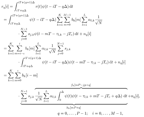
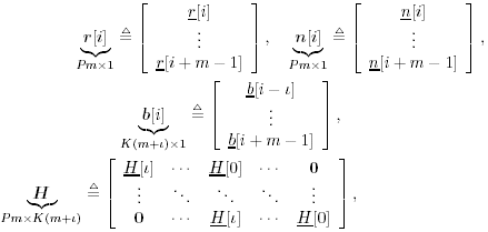
In previous sections we focused on the synchronous CDMA signal model. In a practical wireless CDMA system, however, the users' signals are asynchronous. Moreover, the physical channel exhibits dispersion due to multipath effects that further distort the signals. In this section we address blind multiuser detection in such channels. As will be seen, the principal techniques developed in previous sections can be applied to this more realistic situation as well.

2.7.1 Multipath Signal Model

We now consider a more general multiple-access signal model where the users are asynchronous, and the channel exhibits multipath distortion effects. In particular, the multipath channel impulse response of the k th user is modeled as in (1.10):

Equation 2.165

where L is the total number of paths in the channel, and a _l,k and t _l,k are, respectively, the complex path gain and the delay of the k th user's l th path, t _{1, k} < t _{2, k} < · · · < t _L,k . The continuous-time signal received in this case is given by

Equation 2.166

where * denotes convolution and s _k (t) is the spreading waveform of the k th user given by (2.2).

At the receiver, the received signal r(t) is filtered by a chip-matched filter and sampled at a multiple (p) of the chip rate (i.e., the sampling time interval is D = T _c /p = T/P , where is the total number of samples per symbol interval). Let

be the maximum delay spread in terms of symbol intervals. Substituting (2.2) into (2.166), the q th signal sample during the i th symbol interval is given by!

Equation 2.167

where . Denote

Then (2.167) can be written in terms of vector convolution as

Equation 2.168

By stacking m successive sample vectors, we further define the following quantities :

where the smoothing factor m is chosen according to . Note that for such m , the matrix H is a "tall" matrix [i.e., Pm K(m + I ) ]. We can then write (2.168) in matrix form as

Equation 2.169

2.7.2 Linear Multiuser Detectors

Suppose that we are interested in demodulating the data of user 1. Then (2.168) can be written as

Equation 2.170

where denotes the k th column of . In (2.170), the first term contains the data bit of the desired user at time i ; the second term contains the previous data bits of the desired user [i.e., we have intersymbol interference (ISI)]; and the last term contains the signals from other users [i.e., multiple-access interference (MAI)]. Hence, compared with the synchronous model considered in previous sections, the multipath channel introduces ISI, which together with MAI must be contended with at the receiver. Moreover, the augmented signal model (2.169) is very similar to the synchronous signal model (2.5). We proceed to develop linear receivers for this system.

A linear receiver for this purpose can be represented by a Pm dimensional complex vector , which is correlated with the received signal r [ i ] in (2.169) to obtain

Equation 2.171

The coherent detection rule is then given by

Equation 2.172

and the differential detection rule is given by

Equation 2.173

As before, two forms of such linear detectors are the linear decorrelating detector and the linear minimum mean-square-error (MMSE) detector, which are described next .

Linear Decorrelating Detector

The linear decorrelating detector for user 1 has the form of (2.171) “(2.173) with the weight vector w ₁ = d ₁ , such that both the multiple-access interference (MAI) and the intersymbol interference (ISI) are eliminated completely at the detector output. ^[3]

^[3] In the context of equalization, this detector is known as a zero-forcing equalizer , as noted in Chapter 1.

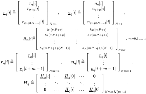
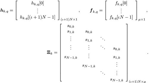
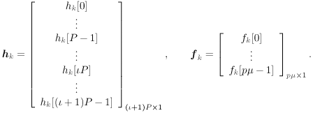
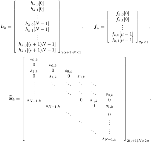
Denote by e _l the K ( m + I )-vector with all-zero entries except for the l th entry, which is 1. Recall that the smoothing factor m is chosen such that the matrix H in (2.169) is a tall matrix. Assume that H has full column rank [i.e., ]. Let H be the Moore “Penrose generalized inverse of the matrix H :

Equation 2.174

The linear decorrelating detector for user 1 is then given by

Equation 2.175

Using (2.169) and (2.175), we have

Equation 2.176

It is seen from (2.176) that both the MAI and the ISI are eliminated completely at the output of the linear zero-forcing detector. In the absence of noise (i.e., n [ i ] = ), the data bit of the desired user, b ₁ [ i ], is recovered perfectly .

Linear MMSE Detector

The linear minimum mean-square-error (MMSE) detector for user 1 has the form of (2.171) “(2.173) with the weight vector w ₁ = m ₁ , where is chosen to minimize the output mean-square error (MSE):

Equation 2.177

where

Equation 2.178

Equation 2.179

Subspace Linear Detectors

Let l ₁ l ₂ · · · l _Pm be the eigenvalues of C _r in (2.178). Since the matrix H has full column rank the signal component of the covariance matrix C _r (i.e., H H ^H ) has rank r . Therefore, we have

By performing an eigendecomposition of the matrix C _r , we obtain

Equation 2.180

where L _s = diag ( l ₁ , ..., l _r ) contains the r largest eigenvalues of C _r in descending order, U _s = [ u ₁ · · · u _r ] contains the corresponding orthogonal eigenvectors, and U _n = [ u _{r +1} · · · u _Pm ] contains the Pm-r orthogonal eigenvectors that correspond to the eigenvalue s ² . It is easy to see that range ( H ) = range ( U _s ). As before, the column space of U _s is called the signal subspace and its orthogonal complement, the noise subspace , is spanned by the columns of U _n .

Following exactly the same line of development as in the synchronous case, it can be shown that the linear decorrelating detector given by (2.175), and the linear MMSE detector given by (2.177), can be expressed in terms of the signal subspace components above as [548]

Equation 2.181

Equation 2.182

Decimation-Combining Linear Detectors

The linear detectors discussed above operate in a Pm -dimensional vector space. As will be seen in the next section, the major computation in channel estimation involves computing the singular value decomposition (SVD) of the autocorrelation matrix C _r of dimensions Pm x Pm , which has computational complexity . By down-sampling the received signal sample vector r [ i ] by a factor of p , it is possible to construct the linear detectors in an Nm -dimensional space and to reduce the total computational complexity of channel estimation by a factor of . (Recall that p is the chip oversampling factor.) This technique is described next.

For q = 0, ..., p - 1, denote

Similar to what we did before, we can write

Equation 2.183

Assume that N _m K(m+ I ) (i.e., the matrix H _q is a tall matrix), and rank ( H _q ) = K ( m + I ) (i.e., H _q has full column rank). For each down-sampled received signal r _q [ i ], the corresponding weight vectors for user 1's linear decorrelating detector and the linear MMSE detector are given, respectively, by

Equation 2.184

Equation 2.185

where . By computing the subspace components of the autocorrelation matrix C _q , subspace versions of the linear detectors above can be constructed in forms similar to (2.181) and (2.182).

To detect user 1's data bits, each down-sampled signal vector r _q [ i ] is correlated with the corresponding weight vector to obtain

Equation 2.186

The data bits are then demodulated according to

Equation 2.187

Equation 2.188

In the decimation-combining approach described above, since the signal vectors have dimension Nm , the complexity of estimating each decimated channel response h _k,q , q = 0, ..., p “1, is . Hence the total complexity of channel estimation is [i.e., a reduction of is achieved compared with the Pm -dimensional detectors]. However, the number of users that can be supported by this receiver structure is reduced by a factor of p . That is, for a given smoothing factor m , the number of users that can be accommodated by the Pm -dimensional detector is , whereas by forming p Nm -dimensional detectors and then combining their outputs, the number of users that can be supported is reduced to .

2.7.3 Blind Channel Estimation

It is seen from the discussion above that unlike the synchronous case, where the linear detectors can be written in closed form once the signal subspace components are identified, in multipath channels the composite channel response vector of the desired user, is needed to form the blind detector. This vector can be viewed as the channel- distorted original spreading waveform s ₁ . The multipath channel can be estimated by transmitting a training sequence [32, 64, 112, 442, 581, 612]. Alternatively, the channel can be estimated blindly by exploiting the orthogonality between the signal and noise subspaces [31, 272, 484, 548, 551]. We next address the problem of blind channel estimation. From (2.167),

Equation 2.189

with

Equation 2.190

where p µ is the length of the channel response { f _k [ m ]},which satisfies

Equation 2.191

Decimate h _k [ n ] into p subsequences as

Equation 2.192

Note that the sequences f _k,q [ m ] are obtained by down-sampling the sequence { f _k [ m ]} by a factor of p :

Equation 2.193

From (2.192), we have

Equation 2.194

Denote

Then (2.194) can be written in matrix form as

Equation 2.195

Finally, denote

Then we have

Equation 2.196

where matrix formed from the signature waveform of the k th user. For instance, when the oversampling factor p = 2, we have

For other values of p , the matrix is constructed similarly.

Recall that when the ambient channel noise is white, through an eigendecomposition on the autocorrelation matrix of the received signal [cf. (2.180)], the signal subspace and the noise subspace can be identified. The channel response f _k can then be estimated by exploiting the orthogonality between the signal subspace and the noise subspace [31, 272, 484, 548]. Specifically, since U _n is orthogonal to the column space of H and is in the column space of H [cf. (2.179)], we have

Equation 2.197

where

Equation 2.198

Based on the relationship above, we can obtain an estimate of the channel response f _k by computing the minimum eigenvector of the matrix . The condition for the channel estimate obtained in such a way to be unique is that the matrix has rank p µ - 1, which necessitates that this matrix be tall (i.e., [ Pm - K ( m + I )] p µ _k ). Since µ I N [cf. (2.191)], we therefore choose the smoothing factor m to satisfy

Equation 2.199

That is, . On the other hand, the condition (2.199) implies that for fixed m , the total number of users that can be accommodated in the system is

Finally, we summarize the batch algorithm for blind linear multiuser detection in multipath CDMA channels as follows .

Algorithm 2.7: [Subspace blind linear multiuser detector ”multipath CDMA]

• Estimate the signal subspace:

Equation 2.200

Equation 2.201

• Estimate the channel and form the detector:

Equation 2.202

Equation 2.203

Equation 2.204

Equation 2.205

• Perform differential detection:

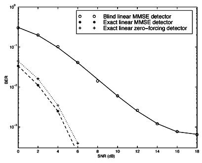
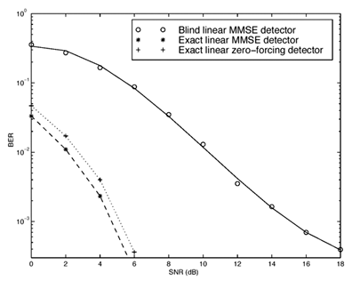
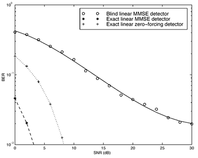
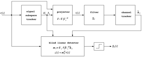
Equation 2.206

Equation 2.207

Alternatively, if the linear receiver has the decimation-combining structure, the noise subspace U _n,q is computed for each q = 0, ..., p - 1. The corresponding channel response f _k,q can then be estimated from the orthogonality relationship

Equation 2.208

Simulation Examples

The simulated system is an asynchronous CDMA system with processing gain N = 15. The m -sequences of length 15 and their shifted versions are employed as the user spreading sequences. The chip pulse is a raised cosine pulse with roll-off factor 0.5. Each user's channel has L = 3 paths. The delay of each path t _l,k is uniformly distributed on [0, 10 T _c ]. Hence the maximum delay spread is one symbol interval (i.e., I = 1). The fading gain of each path in each user's channel is generated from a complex Gaussian distribution and is fixed over the duration of one signal frame. The path gains in each user's channel are normalized so that all users' signals arrive at the receiver with the same power. The oversampling factor is p = 2. The smoothing factor is m = 2. Hence this system can accommodate up to users. If the decimation-combining receiver structure is employed, the maximum number of users is . The length of each user's signal frame is M = 200.

We first consider a five-user system. For the Pm -dimensional implementations , the bit error rates of a particular user incurred by the exact linear MMSE detector, the exact linear zero-forcing detector and the estimated linear MMSE detector are plotted in Fig. 2.13. The bit-error rates of the same user incurred by the three detectors using the decimation-combining structure are plotted in Fig. 2.14. It is seen that for the exact linear zero-forcing and linear MMSE detectors, the performance under the two structures is identical. For the blind linear MMSE receiver, the Pm -dimensional detector achieves an approximately 1-dB performance gain over the decimation-combining detector for SNR in the range 4 to 12 dB. Another observation is that the blind linear MMSE detector tends to exhibit an error floor at high SNR. This is due to the finite length of the signal frame, from which the detector is estimated. Next, a 10-user system is simulated using the Pm -dimensional detectors. The performance of the same user by the three detectors is plotted in Fig. 2.15.

Figure 2.13. Performance of Pm -dimensional linear detectors in a five-user system with white noise.

Figure 2.14. Performance of decimation-combining linear detectors in a five-user system with white noise.

Figure 2.15. Performance of Pm -dimensional linear detectors in a 10-user system with white noise.

2.7.4 Adaptive Receiver Structures

We next consider adaptive algorithms for sequentially estimating the blind linear detector. First, we address adaptive implementation of the blind channel estimator discussed above. Suppose that the signal subspace U _s is known. Denote by z [ i ] the projection of the received signal r [ i ] onto the noise subspace:

Equation 2.209

Equation 2.210

Since z [ i ] lies in the noise subspace, it is orthogonal to any signal in the signal subspace. In particular, it is orthogonal to . Hence f ₁ is the solution to the following constrained optimization problem:

Equation 2.211

In order to obtain a sequential algorithm to solve the optimization problem above, we write it in the following (trivial) state-space form:

The standard Kalman filter can then be applied to the system above, as follows (we define

Equation 2.212

Equation 2.213

Equation 2.214

Note that (2.213) contains a normalization step to satisfy the constraint f ₁ [ i ] = 1.

Since the subspace blind detector may be written in closed form as a function of the signal subspace components, one may use a suitable subspace tracking algorithm in conjuction with this detector and a channel estimator to form an adaptive detector that is able to track changes in the number of users and their composite signature waveforms. Figure 2.16 contains a block diagram of such a receiver. The received signal r [ i ] is fed into a subspace tracker that sequentially estimates the signal subspace components ( U _s , L _s ). The signal r [ i ] is then projected onto the noise subspace to obtain z [ i ], which is in turn passed through a linear filter that is determined by the signature sequence of the desired user. The output of this filter is fed into a channel tracker that estimates the channel state of the desired user. Finally, the linear MMSE detector is constructed in closed form based on the estimated signal subspace components and the channel state. The adaptive receiver algorithm is summarized as follows. Suppose that at time ( i - 1), the estimated signal subspace rank is r [ i - 1] and the components are U _s [ i - 1], L _s [ i - 1], and s ² [ i - 1]. The estimated channel vector is f ₁ [ i - 1]. Then at time i , the adaptive detector performs the following steps to update the detector and estimate the data.

Figure 2.16. Blind adaptive multiuser receiver for multipath CDMA systems.

Algorithm 2.8: [Adaptive blind linear multiuser detector based on subspace tracking ”multipath CDMA]

• Update the signal subspace: Use a particular signal subspace tracking algorithm to update the signal subspace rank r[ i ] and the subspace components U _s [ i ] and L _s [ i ].

• Update the channel: Use (2.212) “(2.214) to update the channel estimate f ₁ [ i ].

• Form the detector and perform differential detection:

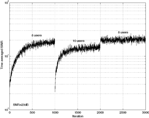
Equation 2.215

Equation 2.216

Equation 2.217

Simulation Example

We next give a simulation example illustrating the performance of the blind adaptive receiver in an asynchronous CDMA system with multipath channels. The processing gain N = 15 and the spreading codes are Gold codes of length 15. Each user's channel has L = 3 paths. The delay of each path t _l,k is uniformly distributed on [0, 10 T _c ]. Hence, as in the preceding example, the maximum delay spread is one symbol interval (i.e., I = 1). The fading gain of each path in each user's channel is generated from a complex Gaussian distribution and is fixed for all simulations. The path gains in each user's channel are normalized so that all users' signals arrive at the receiver with the same power. The smoothing factor is m = 2. The received signal is sampled at twice the chip rate ( p = 2). Hence the total number of users that this system can accommodate is 10. Figure 2.17 shows the performance of subspace blind adaptive receiver using the NAHJ subspace tracking algorithm discussed in Section 2.6.3 in terms of output SINR. During the first 1000 iterations there are eight total users. At iteration 1000, four new users are added to the system. At iteration 2000, one additional known user is added and three existing users vanish . We see that this blind adaptive receiver can closely track the dynamics of the channel.

Figure 2.17. Performance of a subspace blind adaptive multiuser detector in an asynchronous CDMA system with multipath.

We note that there are many other approaches to blind multiuser detection in multipath CDMA channels, such as constrained optimization methods [59, 60, 80, 187, 300, 305, 306, 427, 485, 487, 490, 498, 583, 584, 605], the auxiliary vector method [364],other subspace methods [10, 31, 252, 258, 272, 287, 446, 484, 548, 551, 564], linear prediction methods [69, 117, 207, 606], the multistage Wiener filtering method [156, 186], the constant modulus method [79, 218, 582], the spreading code design method [435], the maximum- likelihood method [56], the parallel factor method [447], the least-squares smoothing method [483, 610], a method based on cyclostationarity [351], and more general methods based on multiple-input /multiple-output (MIMO) blind channel identification [78, 214, 261, 298, 462, 494 “497].

2.7.5 Blind Multiuser Detection in Correlated Noise

So far in developing the subspace-based linear detectors and the channel estimation methods, the ambient channel noise is assumed to be temporally white. In practice, such an assumption may be violated due to, for example, the interference from some narrowband sources. The techniques developed under the white noise assumption are not applicable to channels with correlated ambient noise. In this section we discuss subspace methods for joint suppression of MAI and ISI in multipath CDMA channels with unknown correlated ambient noise, which were first developed in [551]. The key assumption here is that the signal is received by two antennas well separated so that the noise is spatially uncorrelated .

We start with the received augmented discrete-time signal model given by (2.169). Assume that the ambient noise vector n [ i ] has a covariance matrix . Then the Pm x Pm autocorrelation matrix C _r of the received signal r [ i ] is given by

Equation 2.218

The linear MMSE detector m ₁ for user 1 is given by (2.177) with C _r replaced by (2.218). As before, we must first estimate the desired user's composite signature waveform given by (2.198). Notice, however, that when the ambient noise is correlated, it is not possible to separate the signal subspace from the noise subspace based solely on the autocorrelation matrix C _r .

To estimate the channel in unknown correlated noise, we make use of two antennas at the receiver. Then the two augmented received signal vectors at the two antennas can be written, respectively, as

Equation 2.219

Equation 2.220

where H ₁ and H ₂ contain the channel information corresponding to the respective antennas. It is assumed that the two antennas are well separated so that the ambient noise is spatially uncorrelated . In other words, n ₁ [ i ] and n ₂ [ i ] are uncorrelated, and their joint covariance is given by

Equation 2.221

where S ₁ and S ₂ are unknown covariance matrices of the noise at the two antennas. The joint autocorrelation matrix of the received signal at the two antennas is then given by

Equation 2.222

where the submatrices are given by

Equation 2.223

Equation 2.224

Equation 2.225

We next consider two methods for estimating the noise subspaces from the signals received at the two antennas.

Singular Value Decomposition

Assume that both H ₁ and H ₂ have full column rank ; then the matrix C ₁₂ also has rank r . Consider the singular value decomposition of the matrix C ₁₂ ,

Equation 2.226

The Pm x Pm diagonal matrix G has the form G = diag ( g ₁ , ..., g _r , 0, ..., 0), with g ₁ · · · g _r > 0. Now if we partition the matrix U _j as U _j = [ U _j,s U _j,n ] for j = 1, 2, where U _j,s and U _j,n contain the first r columns and the last Pm - r columns of U _j , respectively, the column space of U _j,n is orthogonal to the column space of H _j :

Equation 2.227

where denotes the orthogonal complement space of range ( H _j ). User 1's channel corresponding to antenna j , f _{j ,1} , can then be estimated from the orthogonality relationship

Equation 2.228

Canonical Correlation Decomposition

Assume that the matrices C ₁₁ and C ₂₂ are both positive definite. The canonical correlation decomposition (CCD) of the matrix C ₁₂ is given by [18]

Equation 2.229

or

Equation 2.230

The Pm x Pm matrix G has the form G = diag ( g ₁ , ..., g _r , 0, ..., 0), with g ₁ · · · g _r > 0. Let

Equation 2.231

Partition the matrix L _j such that

Equation 2.232

where L _j,s and L _j,n are the first r columns and the last Pm - r columns of L _j , respectively. The matrix U _j are similarly partitioned into U _j,s and U _j,n . We have [580].

Equation 2.233

Note, however, that L _j,s does not necessarily span the signal subspace range ( H _j ) [580].

Now suppose that we have estimated the composite signature waveform of the desired user , using the identified noise subspace L _j,n . Since , we have

Equation 2.234

where the second equality in (2.234) follows from (2.231) and the fact that U _j is a unitary matrix; and the third equality follows from the fact that .

Let the estimated weight vectors of the linear MMSE detectors at the two antennas be . To make use of the received signal at both antennas, we use the following equal-gain differential combining rule for detecting the differential bit b ₁ [ i ]:

Equation 2.235

Equation 2.236

We next summarize the procedures for computing the linear MMSE detector in unknown correlated noise based on the discussion above. Let

Equation 2.237

be the matrix of M received augmented signal sample vectors at antenna j corresponding to one block of data transmission.

Algorithm 2.9: [Blind linear MMSE detector in multipath CDMA with correlated noise ”SVD-based method]

• Compute the auto- and cross-correlation matrices:

Equation 2.238

• Perform an SVD on to get the noise subspace .

• Compute the composite signature waveforms by solving

Equation 2.239

• Form the linear MMSE detectors:

Equation 2.240

• Perform differential detection according to (2.235) “(2.236).

Algorithm 2.10: [Blind linear MMSE detector in multipath CDMA with correlated noise ”CCD-based method]

• Perform QR decomposition:

Equation 2.241

• Perform an SVD on :

Equation 2.242

• Compute

Equation 2.243

where is an upper triangular matrix.

• Partition . Compute the composite signature waveforms by solving

Equation 2.244

• Form the linear MMSE detectors:

Equation 2.245

• Perform differential detection according to (2.235) “(2.236).

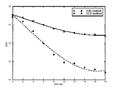
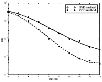
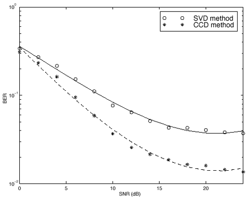
The procedure above is based on the fast algorithm for computing CCD given in [580].

Note that the two methods above operate on the Pm -dimensional signal vectors r _j [ i ], j = 1,2. The same procedures can be applied to the decimated received signal vectors to operate on the Nm -dimensional signal vectors r _j,q [ i ], j = 1,2, q = 0, ..., p - 1. As before, such decimation-combining approach reduces the computational complexity by a factor of . It also reduces the number of users that can be accommodated in the system by a factor of p .

Simulation Examples

We illustrate the performance of the detectors above via simulation examples. The simulated system is the same as that in Section 2.7.3, except that the ambient noise is temporally correlated. The noise at each antenna j is modeled by a second-order autoregressive (AR) model with coefficients a _j = [ a _{j ,1} , a _{j ,2} ]; that is, the noise field is generated according to

Equation 2.246

where n _j [ i ] is the noise at antenna j and sample i , and w _j [ i ] is a complex white Gaussian noise sample with unit variance. The AR coefficients at the two arrays are chosen as a ₁ = [1, -0.2] and a ₂ = [1.2, -0.3].

We first consider a five-user system. In Fig. 2.18 the performance of the Pm -dimensional blind linear MMSE detectors is plotted for both SVD- and CCD-based methods. The corresponding performance by the decimation-combining receiver structure is plotted in Fig. 2.19. Next a 10-user system is simulated and the performance of the Pm -dimensional blind linear MMSE detectors is plotted in Fig. 2.20.

Figure 2.18. Performance of Pm -dimensional blind linear MMSE detectors in a five-user system with correlated noise.

Figure 2.19. Performance of decimation-combining blind linear MMSE detectors in a five-user system with correlated noise.

Figure 2.20. Performance of Pm -dimensional blind linear MMSE detectors in a 10-user system with correlated noise.

It is seen from Figs. 2.18 “2.20 that CCD-based detectors are superior in performance to SVD-based detectors. It has been shown that the CCD has the optimality property of maximizing the correlation between the two sets of linearly transformed data [18]. Maximizing the correlation of the two data sets can yield the best estimate of the correlated (i.e., signal) part of the data. CCD makes use of the information of both and together with and creates the maximum correlation between the two data sets. On the other hand, SVD uses only the information and does not create the maximum correlation between the two data sets, and thus yields inferior performance.