Computer Solution of a Transportation Problem
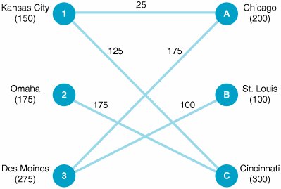
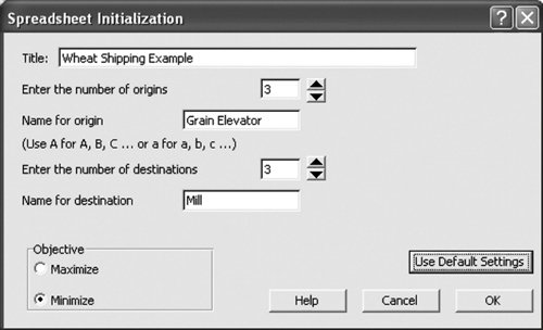
| Because a transportation problem is formulated as a linear programming model, it can be solved with Excel and using the linear programming module of QM for Windows that we introduced in previous chapters. However, management science packages such as QM for Windows also have transportation modules that enable problems to be input in a special transportation tableau format. We will first demonstrate solution of the wheat shipping problem solved earlier in this chapter, this time by using Excel spreadsheets. Computer Solution with ExcelWe will first demonstrate how to solve a transportation problem by using Excel. A transportation problem must be solved in Excel as a linear programming model, using Solver, as demonstrated in Chapters 3 and 4. Exhibit 6.1 shows a spreadsheet setup to solve our wheat-shipping example. Notice that the objective function formula for total cost is contained in cell C10 and is shown on the formula bar at the top of the spreadsheet. It is constructed as a SUMPRODUCT of the decision variables in cells C5:E7 and a cost array in cells K5:M7 . Cells G5:G7 in column G and cells C9:E9 in row 9, labeled "Grain Shipped," contain the constraint formulas for supply and demand, respectively. For example, the constraint formula in cell G7 for the grain shipped from Des Moines to the three mills is =C7+D7+E7 , and the right-hand-side quantity value of 275 available tons is in cell F7. Exhibit 6.1.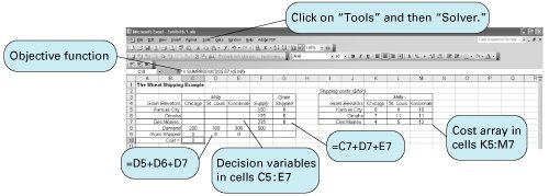 Exhibit 6.2 shows the Solver Parameters screen for our example. Cell C10, containing the objective function formula, is minimized. The constraint formula C9:E9=C8:E8 includes all three demand constraints, and the constraint formula G5:G7=F5:F7 includes all three supply constraints. Before solving this problem, remember to click on "Options" and then, on the resulting screen, click on "Assume Linear Model" to invoke the linear programming solution approach and click on "Assume Non-negative." Exhibit 6.2.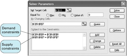 Exhibit 6.3 shows the optimal solution, with the amounts shipped from sources to destinations and the total cost. Figure 6.2 shows a network diagram of the optimal shipments. Exhibit 6.3.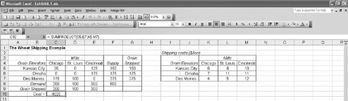 Figure 6.2. Transportation network solution for wheat shipping example Computer Solution with Excel QMExcel QM, which we introduced in Chapter 1, includes a spreadsheet macro for transportation problems. Recall from Chapter 1 that when Excel QM is activated, "QM" is shown on the menu bar at the top of the spreadsheet. Clicking on "QM" and then selecting "Transportation" will result in the Spreadsheet Initialization window appearing, as shown in Exhibit 6.4. In this window we set the number of sources (i.e., origins) and destinations to 3, select "Minimize" as the objective, and type in the title for our example. To exit this window, we click on "OK," and the spreadsheet shown in Exhibit 6.5 is displayed. The transportation problem is completely set up as shown, with all the necessary formulas already in the cells. However, initially the data values in cells B10:E13 are empty; the spreadsheet in Exhibit 6.5 includes the values that we have typed in. Exhibit 6.4. Exhibit 6.5.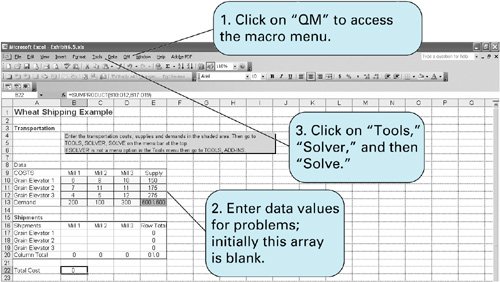 To solve the problem, we follow the instructions in the box superimposed on the spreadsheet in Exhibit 6.5click on "Tools" at the top of the spreadsheet, then click on "Solver," and when Solver appears, click on "Solve." We have not shown the Solver window here; however, it is very similar to the one shown in Exhibit 6.2. It already includes all the decision variables and constraints required to solve the problem; thus, all that is needed is to click on "Solve." The spreadsheet with the solution is shown in Exhibit 6.6. You will notice that although the total cost is the same as in the solution we obtained with Excel in Exhibit 6.3, the decision variable values in cells B17:D19 are different. This is because this problem has multiple optimal solutions, and this is an alternate solution to the one we got previously. Exhibit 6.6.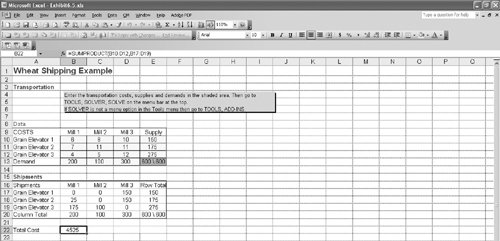 QM for Windows SolutionTo access the transportation module for QM for Windows, click on "Module" at the top of the screen and then click on "Transportation." Once you are in the transportation module, click on "File" and then "New" to input the problem data. QM for Windows allows for any of three initial solution methodsnorthwest corner, minimum cell cost, or VAMto be selected. These are the three starting solution procedures used in the mathematical procedure for solving transportation problems. Because these techniques are not included in the text (but are included on the accompanying CD), it makes no difference which starting procedure we use. Exhibit 6.7 shows the input data for our wheat shipping example. Exhibit 6.7.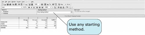 Once the data are input, clicking on "Solve" at the top of the screen will generate the solution, as shown in Exhibits 6.8 and 6.9. QM for Windows will indicate if multiple optimal solutions exist, but it will not identify alternate solutions. This is the same optimal solution that we achieved earlier in our Excel QM solution. Exhibits 6.8 and 6.9 show the solution results in two different tables, or formats. Exhibit 6.8 shows the shipments in each cell (or decision variable) plus total cost, while Exhibit 6.9 lists the individual shipments from each source to destination and their costs. Exhibit 6.8. Exhibit 6.9.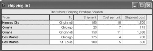 |
EAN: 2147483647
Pages: 358