The Transportation Model
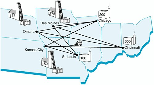
| The transportation model is formulated for a class of problems with the following unique characteristics: (1) A product is transported from a number of sources to a number of destinations at the minimum possible cost; and (2) each source is able to supply a fixed number of units of the product, and each destination has a fixed demand for the product. Although the general transportation model can be applied to a wide variety of problems, it is this particular application to the transportation of goods that is most familiar and from which the problem draws its name . In a transportation problem , items are allocated from sources to destinations at a minimum cost . The following example demonstrates the formulation of the transportation model. Wheat is harvested in the Midwest and stored in grain elevators in three different citiesKansas City, Omaha, and Des Moines. These grain elevators supply three flour mills, located in Chicago, St. Louis, and Cincinnati. Grain is shipped to the mills in railroad cars, each car capable of holding 1 ton of wheat. Each grain elevator is able to supply the following number of tons (i.e., railroad cars ) of wheat to the mills on a monthly basis:
Each mill demands the following number of tons of wheat per month:
The cost of transporting 1 ton of wheat from each grain elevator (source) to each mill (destination) differs , according to the distance and rail system. (For example, the cost of shipping 1 ton of wheat from the grain elevator at Omaha to the mill at Chicago is $7.) These costs are shown in the following table:
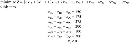
The problem is to determine how many tons of wheat to transport from each grain elevator to each mill on a monthly basis to minimize the total cost of transportation. A diagram of the different transportation routes, with supply and demand, is given in Figure 6.1. The linear programming model for a transportation problem has constraints for supply at each source and demand at each destination . Figure 6.1. Network of transportation routes for wheat shipments The linear programming model for this problem is formulated as follows : In this model the decision variables , x ij , represent the number of tons of wheat transported from each grain elevator, i (where i = 1, 2, 3), to each mill, j (where j = A, B, C). The objective function represents the total transportation cost for each route. Each term in the objective function reflects the cost of the tonnage transported for one route. For example, if 20 tons are transported from elevator 1 to mill A, the cost ($6) is multiplied by x 1A (= 20), which equals $120. The first three constraints in the linear programming model represent the supply at each elevator; the last three constraints represent the demand at each mill. As an example, consider the first supply constraint, x 1A + x 1B + x 1C = 150. This constraint represents the tons of wheat transported from Kansas City to all three mills: Chicago ( x 1A ), St. Louis ( x 1B ), and Cincinnati ( x 1C ). The amount transported from Kansas City is limited to the 150 tons available. Note that this constraint (as well as all others) is an equation (=) rather than a In a balanced transportation model in which supply equals demand, all constraints are equalities . Realistically, however, an unbalanced problem , in which supply exceeds demand or demand exceeds supply, is a more likely occurrence. In our wheat transportation example, if the demand at Cincinnati is increased from 300 tons to 350 tons, a situation is created in which total demand is 650 tons and total supply is 600 tons. This would result in the following change in our linear programming model of this problem: One of the demand constraints will not be met because there is not enough total supply to meet total demand. If, instead, supply exceeds demand, then the supply constraints would be Sometimes one or more of the routes in the transportation model may be prohibited . That is, units cannot be transported from a particular source to a particular destination. When this situation occurs, we must make sure that the variable representing that route does not have a value in the optimal solution. This can be accomplished by assigning a very large relative cost as the coefficient of this prohibited variable in the objective function. For example, in our wheat-shipping example, if the route from Kansas City to Chicago is prohibited (perhaps because of a rail strike), the variable x 1A is given a coefficient of 100 instead of 6 in the objective function, so x 1A will equal zero in the optimal solution because of its high relative cost. Alternatively the prohibited variable can be deleted from the model formulation.
| ||||||||||||||||||||||||||||||||||||||||||
 inequality because all the tons of wheat available will be needed to meet the
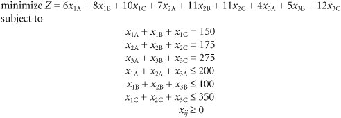
EAN: 2147483647
Pages: 358