The Transshipment Model

[Page 230 ( continued )]

The transshipment model is an extension of the transportation model in which intermediate transshipment points are added between the sources and destinations. An example of a transshipment point is a distribution center or warehouse located between plants and stores. In a transshipment problem, items may be transported from sources through transshipment points on to destinations, from one source to another, from one transshipment point to another, from one destination to another, or directly from sources to destinations, or some combination of these alternatives.

[Page 231]

The transshipment model includes intermediate points between sources and destinations .

We will expand our wheat shipping example to demonstrate the formulation of a transshipment model. Wheat is harvested at farms in Nebraska and Colorado before being shipped to the three grain elevators in Kansas City, Omaha, and Des Moines, which are now transshipment points. The amount of wheat harvested at each farm is 300 tons. The wheat is then shipped to the mills in Chicago, St. Louis, and Cincinnati. The shipping costs from the grain elevators to the mills remain the same, and the shipping costs from the farms to the grain elevators are as follows :

	Grain Elevator
Farm	3. K ANSAS C ITY	4. O MAHA	5. D ES M OINES
1. Nebraska	$16	$10	$12
2. Colorado	15	14	17

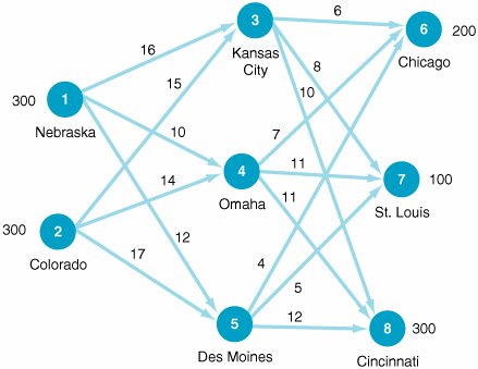
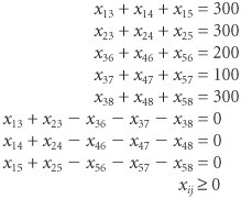
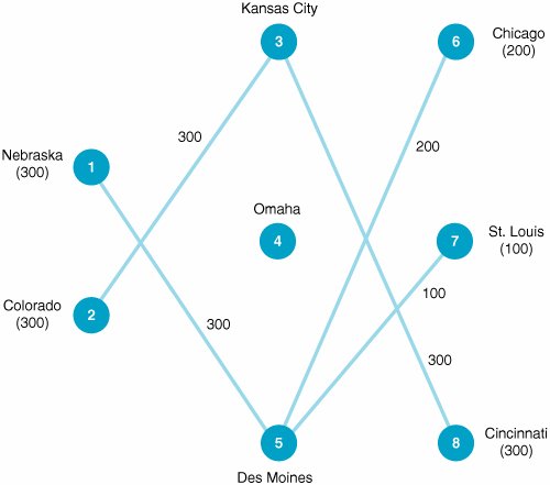
The basic structure of this model is shown in the graphical network in Figure 6.3.

Figure 6.3. Network of transshipment routes

As with the transportation problem, a linear programming model is developed with supply and demand constraints. The available supply constraints for the farms in Nebraska and Colorado are

x ₁₃ + x ₁₄ + x ₁₅ = 300

x ₂₃ + x ₂₄ + x ₂₅ = 300

The demand constraints at the Chicago, St. Louis, and Cincinnati mills are

x ₃₆ + x ₄₆ + x ₅₆ = 200

x ₃₇ + x ₄₇ + x ₅₇ = 100

x ₃₈ + x ₄₈ + x ₅₈ = 300

Next we must develop constraints for the grain elevators (i.e., transshipment points) at Kansas City, Omaha, and Des Moines. To develop these constraints we follow the principle that at each transshipment point, the amount of grain shipped in must also be shipped out . For example, the amount of grain shipped into Kansas City is

[Page 232]

x ₁₃ + x ₂₃

and the amount shipped out is

x ₃₆ + x ₃₇ + x ₃₈

Thus, because whatever is shipped in must also be shipped out, these two amounts must equal each other:

x ₁₃ + x ₂₃ = x ₃₆ + x ₃₇ + x ₃₈

x ₁₃ + x ₂₃ x ₃₆ x ₃₇ x ₃₈ = 0

The transshipment constraints for Omaha and Des Moines are constructed similarly:

x ₁₄ + x ₂₄ x ₄₆ x ₄₇ x ₄₈ = 0

x ₁₅ + x ₂₅ x ₅₆ x ₅₇ x ₅₈ = 0

The complete linear programming model, including the objective function, is summarized as follows:

minimize Z	=	$16 x ₁₃ + 10 x ₁₄ + 12 x ₁₅ + 15 x ₂₃ + 14 x ₂₄ + 17 x ₂₅ + 6 x ₃₆ + 8 x ₃₇ + 10 x ₃₈
		+ 7 x ₄₆ + 11 x ₄₇ + 11x ₄₈ + 4x ₅₆ + 5 x ₅₇ + 12 x ₅₈
subject to

Computer Solution with Excel

Because the transshipment model is formulated as a linear programming model, it can be solved with either Excel or QM for Windows. Here we will demonstrate its solution with Excel.

Exhibit 6.10 shows the spreadsheet solution and Exhibit 6.11 the solver for our wheat shipping transshipment example. A network diagram of the optimal solution is shown in Figure 6.4. The spreadsheet is similar to the original spreadsheet for the regular transportation problem in Exhibit 6.1 except that there are two tables of variablesone for shipping from the farms to the grain elevators and one for shipping grain from the elevators to the mills. Thus, the decision variables (i.e., the amounts shipped from sources to destinations) are in cells B6:D7 and C13:E15 . The constraint for the amount of grain shipped from the farm in Nebraska to the three grain elevators (i.e., the supply constraint for Nebraska) in cell F6 is =SUM(B6:D6) , which sums cells B6+C6+D6 . The amount of grain shipped to Kansas City from the farms in cell B8 is =SUM(B6:B7) . Similar constraints are developed for the shipments from the grain elevators to the mills.

[Page 233]

Exhibit 6.10.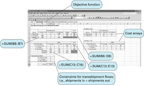

Exhibit 6.11.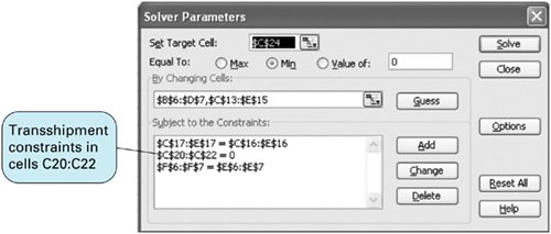

Two cost arrays have been developed for the shipping costs in cells I6:K7 and cells J13:L15 , which are then multiplied by the variables in cells B6:D7 and C13:E15 and added together. The objective function, =SUMPRODUCT(B6:D7,I6:K7)+SUMPRODUCT(C13:E15,J13:L15) , is shown on the toolbar at the top of Exhibit 6.10. Constructing the objective function with cost arrays like this is a little easier than typing in all the variables and costs in a single objective function when there are a lot of variables and costs.

[Page 234]

The Transshipment Model