Converting the Model into Standard Form
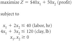
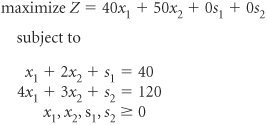
| The first step in solving a linear programming model manually with the simplex method is to convert the model into standard form. At the Beaver Creek Pottery Company Native American artisans produce bowls ( x 1 ) and mugs ( x 2 ) from labor and clay. The linear programming model is formulated as We convert this model into standard form by adding slack variables to each constraint as follows . The slack variables, s 1 and s 2 , represent the amount of unused labor and clay, respectively. For example, if no bowls and mugs are produced, and x 1 = 0 and x 2 = 0, then the solution to the problem is
and
Slack variables are added to In other words, when we start the problem and nothing is being produced, all the resources are unused. Since unused resources contribute nothing to profit, the profit is zero.
It is at this point that we begin to apply the simplex method. The model is in the required form, with the inequality constraints converted to equations for solution with the simplex method. The Solution of Simultaneous EquationsOnce both model constraints have been transformed into equations, the equations should be solved simultaneously to determine the values of the variables at every possible solution point. However, notice that our example problem has two equations and four unknowns (i.e., two decision variables and two slack variables), a situation that makes direct simultaneous solution impossible . The simplex method alleviates this problem by assigning some of the variables a value of zero. The number of variables assigned values of zero is n m , where n equals the number of variables and m equals the number of constraints (excluding the nonnegativity constraints). For this model, n = 4 variables and m = 2 constraints; therefore, two of the variables are assigned a value of zero (i.e., 4 2 = 2). For example, letting x 1 = 0 and s 1 = 0 results in the following set of equations.
and
First, solve for x 2 in the first equation:
Then, solve for s 2 in the second equation:
This solution corresponds with point A in Figure A-1. The graph in Figure A-1 shows that at point A , x 1 = 0, x 2 = 20, s 1 = 0, and s 2 = 60, the exact solution obtained by solving simultaneous equations. This solution is referred to as a basic feasible solution . A feasible solution is any solution that satisfies the constraints. A basic feasible solution satisfies the constraints and contains as many variables with nonnegative values as there are model constraintsthat is, m variables with nonnegative values and n m values set equal to zero. Typically, the m variables have positive nonzero solution values; however, when one of the m variables equals zero, the basic feasible solution is said to be degenerate . (The topic of degeneracy will be discussed at a later point in this module.) Figure A-1. Solutions at points A , B , and C A basic feasible solution satisfies the model constraints and has the same number of variables with non-negative values as there are constraints. Consider a second example where x 2 = 0 and s 2 = 0. These values result in the following set of equations.
and
Solve for x 1 :
Then solve for s 1 :
This basic feasible solution corresponds to point C in Figure A-1, where x 1 = 30, x 2 = 0, s 1 = 10, and s 2 = 0. Finally, consider an example where s 1 = 0 and s 2 = 0. These values result in the following set of equations.
and
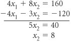
These equations can be solved using row operations . In row operations, the equations can be multiplied by constant values and then added or subtracted from each other without changing the values of the decision variables. First, multiply the top equation by 4 to get 4 x 1 + 8 x 2 = 160 and then subtract the second equation: Next, substitute this value of x 2 into either one of the constraints.
Row operations are used to solve simultaneous equations where equations are multiplied by constants and added or subtracted from each other. This solution corresponds to point B on the graph, where x 1 = 24, x 2 = 8, s 1 = 0, and s 2 = 0, which is the optimal solution point. All three of these example solutions meet our definition of basic feasible solutions . However, two specific questions are raised by the identification of these solutions.
The answers to both of these questions can be found by using the simplex method. The simplex method is a set of mathematical steps that determines at each step which variables should equal zero and when an optimal solution has been reached. |
 constraints and represent unused resources.
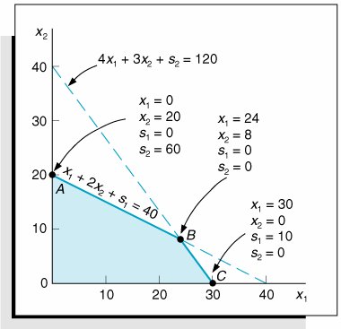
EAN: 2147483647
Pages: 358