A Minimization Model Example
| As mentioned at the beginning of this chapter, there are two types of linear programming problems: maximization problems (like the Beaver Creek Pottery Company example) and minimization problems. A minimization problem is formulated the same basic way as a maximization problem, except for a few minor differences. The following sample problem will demonstrate the formulation of a minimization model. A farmer is preparing to plant a crop in the spring and needs to fertilize a field. There are two brands of fertilizer to choose from, Super-gro and Crop-quick. Each brand yields a specific amount of nitrogen and phosphate per bag, as follows :
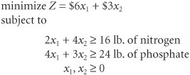
The farmer's field requires at least 16 pounds of nitrogen and 24 pounds of phosphate. Super-gro costs $6 per bag, and Crop-quick costs $3. The farmer wants to know how many bags of each brand to purchase in order to minimize the total cost of fertilizing. This scenario is illustrated in Figure 2.15. The steps in the linear programming model formulation process are summarized as follows:
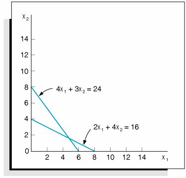
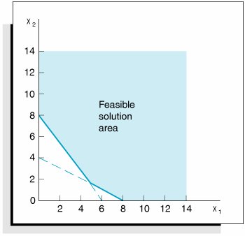
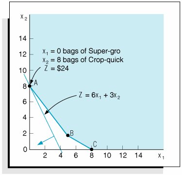
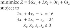
Decision VariablesThis problem contains two decision variables, representing the number of bags of each brand of fertilizer to purchase: x 1 = bags of Super-gro x 2 = bags of Crop-quick Figure 2.15. Fertilizing farmer's field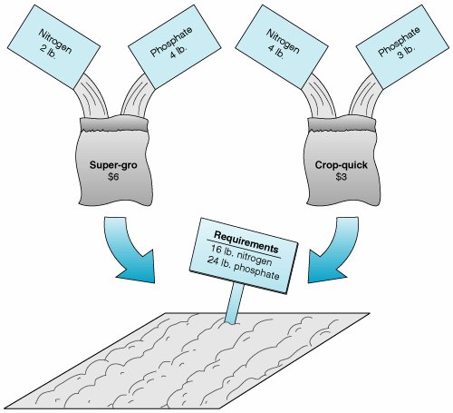 The Objective FunctionThe farmer's objective is to minimize the total cost of fertilizing. The total cost is the sum of the individual costs of each type of fertilizer purchased. The objective function that represents total cost is expressed as minimize Z = $6 x 1 + 3 x 2 where $6 x 1 = cost of bags of Super-gro $3 x 2 = cost of bags of Crop-quick Model ConstraintsThe requirements for nitrogen and phosphate represent the constraints of the model. Each bag of fertilizer contributes a number of pounds of nitrogen and phosphate to the field. The constraint for nitrogen is 2 x 1 + 4 x 2 where 2 x 1 = the nitrogen contribution (lb.) per bag of Super-gro 4 x 2 = the nitrogen contribution (lb.) per bag of Crop-quick Rather than a The constraint for phosphate is constructed like the constraint for nitrogen: 4 x 1 + 3 x 2 With this example we have shown two of the three types of linear programming model constraints, The three types of linear programming constraints are 4 x 1 + 3 x 2 = 24 lb. As in our maximization model, there are also nonnegativity constraints in this problem to indicate that negative bags of fertilizer cannot be purchased: x 1 , x 2 The complete model formulation for this minimization problem is Graphical Solution of a Minimization ModelWe follow the same basic steps in the graphical solution of a minimization model as in a maximization model. The fertilizer example will be used to demonstrate the graphical solution of a minimization model. The first step is to graph the equations of the two model constraints, as shown in Figure 2.16. Next, the feasible solution area is chosen , to reflect the Figure 2.16. Constraint lines for fertilizer model Figure 2.17. Feasible solution area After the feasible solution area has been determined, the second step in the graphical solution approach is to locate the optimal point. Recall that in a maximization problem, the optimal solution is on the boundary of the feasible solution area that contains the point(s) farthest from the origin. The optimal solution point in a minimization problem is also on the boundary of the feasible solution area; however, the boundary contains the point(s) closest to the origin (zero being the lowest cost possible). The optimal solution of a minimization problem is at the extreme point closest to the origin . As in a maximization problem, the optimal solution is located at one of the extreme points of the boundary. In this case the corner points represent extremities in the boundary of the feasible solution area that are closest to the origin. Figure 2.18 shows the three corner points A , B , and C and the objective function line. As the objective function edges toward the origin, the last point it touches in the feasible solution area is A . In other words, point A is the closest the objective function can get to the origin without encompassing infeasible points. Thus, it corresponds to the lowest cost that can be attained. Figure 2.18. The optimal solution point
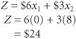
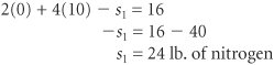
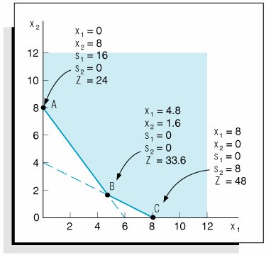
The final step in the graphical solution approach is to solve for the values of x 1 and x 2 at point A . Because point A is on the x 2 axis, x 1 = 0; thus, Given that the optimal solution is x 1 = 0, x 2 = 8, the minimum cost, Z , is This means the farmer should not purchase any Super-gro but, instead, should purchase eight bags of Crop-quick, at a total cost of $24. Surplus Variables Greater than or equal to constraints cannot be converted to equations by adding slack variables, as with where x 1 = bags of Super-gro fertilizer x 2 = bags of Crop-quick fertilizer Z = farmer's total cost ($) of purchasing fertilizer Because this problem has A surplus variable is subtracted from a Instead of adding a slack variable with a For the nitrogen constraint, the subtraction of a surplus variable gives A surplus variable represents an excess above a constraint requirement level . 2 x 1 + 4 x 2 s 1 = 16 The surplus variable s 1 transforms the nitrogen constraint into an equation. As an example, consider the hypothetical solution x 1 = 0 x 2 = 10 Substituting these values into the previous equation yields In this equation s 1 can be interpreted as the extra amount of nitrogen above the minimum requirement of 16 pounds that would be obtained by purchasing 10 bags of Crop-quick fertilizer. In a similar manner, the constraint for phosphate is converted to an equation by subtracting a surplus variable, s 2 : 4 x 1 + 3 x 2 s 2 = 24 Figure 2.19. Graph of the fertilizer example As is the case with slack variables, surplus variables contribute nothing to the overall cost of a model. For example, putting additional nitrogen or phosphate on the field will not affect the farmer's cost; the only thing affecting cost is the number of bags of fertilizer purchased. As such, the standard form of this linear programming model is summarized as Figure 2.19 shows the graphical solutions for our example, with surplus variables included at each solution point. | ||||||||||||||||||||
 16 lb.
  (less than or equal to) inequality, as used in the Beaver Creek Pottery Company model, this constraint requires a
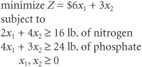

EAN: 2147483647
Pages: 358