Formulating the CPMPERT Network as a Linear Programming Model
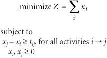
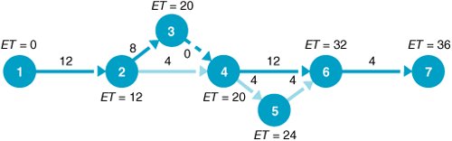
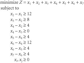
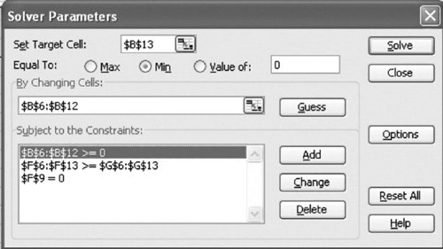
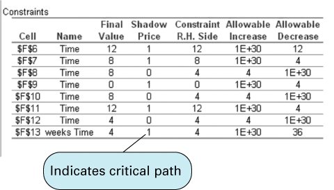
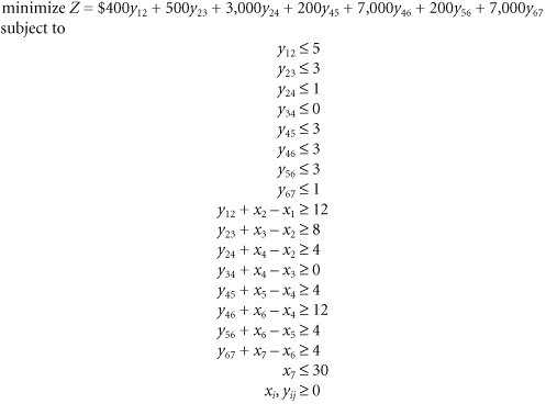
Formulating the CPM/PERT Network as a Linear Programming ModelFirst we will look at the linear programming formulation of the general CPM/PERT network model and then at the formulation of the project crashing network. We will formulate the linear programming model of a CPM/PERT network, using the AOA convention. As the first step in formulating the linear programming model, we will define the decision variables . In our discussion of CPM/PERT networks using the AOA convention, we designated an activity by its start and ending node numbers . Thus, an activity starting at node 1 and ending at node 2 was referred to as activity 1 We will use a different scheduling convention. Instead of determining the earliest activity start time for each activity, we will use the earliest event time at each node. This is the earliest time that a node ( i or j ) can be realized. In other words, it is the earliest time that the event the node represents, either the completion of all the activities leading into it or the start of all activities leaving it, can occur. Thus, for an activity i The objective function for the linear programming model is to minimize project duration. The objective of the project network is to determine the earliest time the project can be completed (i.e., the critical path time). We have already determined from our discussion of CPM/PERT network analysis that the earliest event time of the last node in the network equals the critical path time. If we let x i equal the earliest event times of the nodes in the network, then the objective function can be expressed as Because the value of Z is the sum of all the earliest event times, it has no real meaning; however, it will ensure the earliest event time at each node. Next , we must develop the model constraints. We will define the time for activity i x j x i The general linear programming model of formulation of a CPM/PERT network can be summarized as where x i = earliest event time of node i x j = earliest event time of node j t ij = time of activity i The solution of this linear programming model will indicate the earliest event time of each node in the network and the project duration. As an example of the linear programming model formulation and solution of a project network, we will use the house-building network that we used to demonstrate project crashing. This network, with activity times in weeks and earliest event times, is shown in Figure 8.24. Figure 8.24. CPM/PERT network for the house-building project, with earliest event times The linear programming model for the network in Figure 8.24 is Notice in this model that there is a constraint for each activity in the network. Solution of the CPM/PERT Linear Programming Model with Excel The linear programming model of the CPM/PERT network in the preceding section enables us to use Excel to schedule the project. Exhibit 8.17 shows an Excel spreadsheet set up to determine the earliest event times for each nodethat is, the x i and x j values in our linear programming model for our house-building example. The earliest start times are in cells B6:B12 . Cells F6:F13 contain the model constraints. For example, cell F6 contains the constraint formula =B7B6 , and cell F7 contains the formula =B8B7 . These constraint formulas will be set Exhibit 8.17.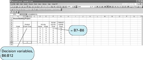 Solver is accessed from the "Tools" menu located at the top of the spreadsheet. The Solver Parameters window with the model data is shown in Exhibit 8.18. Notice that the objective is to minimize the project duration in cell B13, which actually contains the earliest event time for node 7. Exhibit 8.18. The solution is shown in Exhibit 8.19. Notice that the earliest time at each node is given in cells B6:B12 , and the total project duration is 36 weeks. However, this output does not indicate the critical path. The critical path can be determined by accessing the sensitivity report for this problem. Recall that when you click on "Solve" from Solver, a screen comes up, indicating that Solver has reached a solution. This screen also provides the opportunity to generate several different kinds of reports , including an answer report and a sensitivity report. When we click on "Sensitivity" under the report options, the information shown in Exhibit 8.20 is provided. Exhibit 8.19. Exhibit 8.20. The information in which we are interested is the shadow price for each of the activity constraints. (Remember that to get the shadow prices on the sensitivity report, you must click on "Options" from Solver and then select "Assume Linear Model." This is covered in Chapter 3, on solving linear programming problems with Excel.) The shadow price for each activity will be either 1 or 0. A positive shadow price of 1 for an activity means that you can reduce the overall project duration by an amount with a corresponding decrease by the same amount in the activity duration. Alternatively, a shadow price of 0 means that the project duration will not change, even if you change the activity duration by some amount. This means that those activities with a shadow price of 1 are on the critical path. Cells F6, F7, F9, F11, and F13 have shadow prices of 1, and referring back to Exhibit 8.19, we see that these cells correspond to activities 1 Project Crashing with Linear ProgrammingThe linear programming model required to perform project crashing analysis differs from the linear programming model formulated for the general CPM/PERT network in the previous section. The linear programming model for project crashing is somewhat longer and more complex. The objective of the project crashing model is to minimize the cost of crashing . The objective for our general linear programming model was to minimize project duration; the objective of project crashing is to minimize the cost of crashing, given the limits on how much individual activities can be crashed. As a result, the general linear programming model formulation must be expanded to include crash times and cost. We will continue to define the earliest event times for activity i x i = earliest event time of node i x j = earliest event time of node j y ij = amount of time by which activity i The objective of project crashing is to reduce the project duration at the minimum possible crash cost. For our house-building network, the objective function is written as minimize Z = $400 y 12 + 500 y 23 + 3,000 y 24 + 200 y 45 + 7,000 y 46 + 200 y 56 + 7,000 y 67 The objective function coefficients are the activity crash costs per week from Table 8.4; the variables y ij indicate the number of weeks each activity will be reduced. For example, if activity 1 The model constraints must specify the limits on the amount of time each activity can be crashed. Using the allowable crash times for each activity from Table 8.4 enables us to develop the following set of constraints:
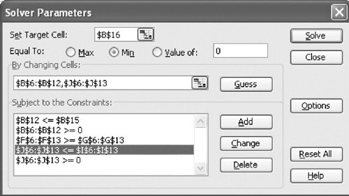
For example, the first constraint, y 12 The next group of constraints must mathematically represent the relationship between earliest event times for each activity in the network, as the constraint x j x i x 2 x 1 This constraint can also be written as x 1 + 12 This latter constraint indicates that the earliest event time at node 1 ( x 1 ), plus the normal activity time (12 weeks) cannot exceed the earliest event time at node 2 ( x 2 ). To reflect the fact that this activity can be crashed, it is necessary only to subtract the amount by which it can be crashed from the left-hand side of the preceding constraint: This revised constraint now indicates that the earliest event time at node 2 ( x 2 ) is determined not only by the earliest event time at node 1 plus the activity time but also by the amount the activity is crashed. Each activity in the network must have a similar constraint, as follows : Finally, we must indicate the project duration we are seeking (i.e., the crashed project time). Because the housing contractor wants to crash the project from the 36-week normal critical path time to 30 weeks, our final model constraint specifies that the earliest event time at node 7 should not exceed 30 weeks: x 7 The complete linear programming model formulation is summarized as follows: Project Crashing with Excel Because we have been able to develop a linear programming model for project crashing, we can also solve this model by using Excel. Exhibit 8.21 shows a modified version of the Excel spreadsheet we developed earlier, in Exhibit 8.16, to determine the earliest event times for our CPM/PERT network for the house-building project. We have added columns H, I, and J for the activity crash costs, the activity crash times, and the actual activity crash times. Cells J6:J13 correspond to the y ij variables in the linear programming model. The constraint formulas for each activity are included in cells F6:F13 . For example, cell F6 contains the formula =J6+B7B6 , and cell F7 contains the formula =J7+B8B7 . These constraints and the others in column F must be set Exhibit 8.21. The problem in Exhibit 8.21 is solved by using Solver, as shown in Exhibit 8.22. Notice that there are two sets of variables in cells B6:B12 and J6:J13 . The project crashing solution is shown in Exhibit 8.23. Exhibit 8.22. Exhibit 8.23. |
 2. We will use a similar designation to define the decision variables of our linear programming model.
 5
5 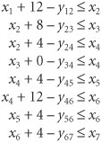
EAN: 2147483647
Pages: 358