1.2 Term structure equation

Equation (1.5) implies that the bond price P = P ( r ( t ), t , T ) is a function of the short rate. Applying Ito's Lemma to the bond price and using (1.4) we derive the stochastic differential equation for the bond price:

Set

and hence

where ¼ ( t , T ) and ƒ ² ( t , T ) are the time t mean and variance of the instantaneous rate of return of a T -maturity zero coupon bond.

Since a single state variable is used to determine all bond prices, the instantaneous returns on bonds of varying maturities are perfectly correlated. Hence a portfolio of positions in two bonds with different maturity dates can be made instantaneously risk-free. This means that the instantaneous return on the portfolio will be the risk-free rate of interest. Consider a time t portfolio of a short position in V ₁ bonds with maturity T ₁ and a long position in V ₂ bonds with maturity T ₂ . The change over time in the value of the portfolio, V = V ₂ ˆ’ V ₁ , is obtained from (1.9):

Choosing V ₁ and V ₂ such that the coefficient of the Wiener coefficient in (1.10) reduces to zero will result in a portfolio with a strictly deterministic instantaneous return. Hence we require:

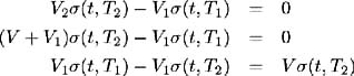
Similarly:

and hence (1.10) becomes:

Invoking assumption 3, that no riskless arbitrage is possible, the instantaneous return on the portfolio must be the risk-free rate, r ( t ). That is:

Rearranging the terms in the equation, we have:

and since this equality is independent of the bond maturity dates, T ₁ and T ₂ , we can define:

where q ( r , t ) is independent of T . q ( r , t ) measures the increase in expected instantaneous return on a bond, for a unit increase in risk, and is referred to as the market price of risk. Substituting the formulae for ¼ and ƒ from (1.7) and (1.8), we derive a partial differential equation for the bond price:

This equation, referred to as the term structure equation, is a general zero coupon bond pricing equation in a market characterised by assumptions 1, 2 and 3. To solve (1.13), we need to specify the parameters of the short-term interest rate process defined by (1.4), the market price of risk q ( r , t ), and apply the boundary condition:

Using equation (1.1) we can evaluate the entire term structure, R ( t , ).