Chapter 12: Time Series and Forecasting

Forecasting is very difficult but essential in any business. Most forecasts are based on past history, and there lies one of the problems. There is no guarantee that the past will repeat itself. Another, of course, is the introduction of changes that will certainly change the outcome of the expectations. Practically all forecasts get these two principles wrong and, as a consequence, statisticians depend on the confidence levels of the forecast to save face. This chapter will introduce the reader to time series and forecasting in a cursory way. Specifically, it will cover autocorrelation, exponential trends, curve smoothing, and econometric models.

EXTRAPOLATION METHODS

Extrapolation methods are quantitative methods that use past data to forecast the future. Primarily, this form of analysis depends on the identification of patterns in the data with the hope that these patterns will be able to be projected into the future. Sometimes, these patterns are controlled by seasonal patterns or known cycles.

Although the effectiveness of extrapolation methods is not yet proven (Armstrong, 1986; Schnarrs and Bavuso, 1986), these methods are extensively used. The reason for their use is that we all want to predict what may happen in some future time given some facts ” never mind that these facts are more often than not dynamic and that they change our expected results, every time.

EXPONENTIAL TREND

Previously we saw that in a linear relationship we can forecast future expectations based on regression modeling. In contrast to a linear trend, an exponential trend is appropriate when the time series changes by a constant percentage (as opposed to a constant such as dollar amount) each period. Then the appropriate regression equation is

Y _t = ce ^bt u _t

where c and b are constants and u represents a multiplicative error term . By taking logarithms of both sides, and letting a = ln(c) and µ _t = ln(u _t ), we obtain a linear equation that can be estimated by the usual linear regression method. However, note that the response variable is now the logarithm of Y _t :

ln( Y _t ) = a + b _t + µ _t

Because the computer does the calculations, our main responsibility is to interpret the final result. This is not too difficult. It can be shown that the coefficient b ( expressed as a percentage) is approximately the percentage change per period. For example, if b = .05, then the series is increasing by approximately 5% per period. On the other hand, if b = -.05, then the series is decreasing by approximately 5% per period. An exponential trend can be estimated with a regression procedure (simple or multiple, whichever you prefer), but only after the log transformation has been made on Y _t . Figure 12.1 shows a hypothetical sales example of a time series with (a) linear trend superimposed, (b) time series of forecast errors, and (c) time series of hypothetical sales with exponential trend superimposed.

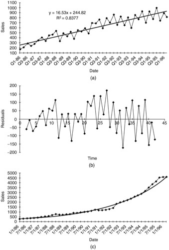
Figure 12.1: Time series plots.

The output shows that there is some evidence of not enough runs. The expected number of runs under randomness is 24.833, and there are only 20 runs for this series. However, the evidence is certainly not overwhelming ” the p-value is only .155. If we ran this test as a one-tailed test, checking only for too few runs, then the appropriate p-value would be .078, half of the value. The conclusion in either case is that sales do not tend to " zigzag " as much as a random series would ” highs tend to follow highs and lows tend to follow lows ” but the evidence in favor of nonrandomness is not overwhelming.

AUTOCORRELATION

The successive observations in a random series are probabilistically independent of one another. Many time series violate this property and are instead autocorrelated. The "auto" means that successive observations are correlated with one other. For example, in the most common form of autocorrelation, positive autocorrelation, large observations tend to follow large observations, and small observations tend to follow small observations. In this case the runs test is likely to pick it up because there will be fewer runs than expected, and the corresponding Z-value for the runs test will be significantly negative. Another way to check for the same nonrandomness property is to calculate the autocorrelations of the time series.

To understand autocorrelations it is first necessary to understand what it means to lag a time series. This concept is easy to understand in spreadsheets. Imagine you are looking at a spreadsheet for sales. To lag by 1 month, we simply "push down" the series by one row; to lag by 2 months, we push down the series by two rows; to lag by 3 months, we push down the series by three rows. Figure 12.2 shows that flow.

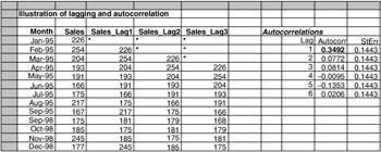
Figure 12.2: Lags and autocorrelation for product X (sales).

See column C of Figure 12.2. Note that there is a blank cell at the top of the lagged series (in cell C4). We can continue to push the series down one row at a time to obtain other lags. For example, the lag 3 version of the series appears in the range E7:E54. Now there are three missing observations at the top. Note that in December 1995, say, the first, second, and third lags correspond to the observations in November 1995, October 1995, and September 1995, respectively. That is, lags are simply previous observations, removed by a certain number of periods from the present time.

In general, the lag k observation corresponding to period t is Y _t-k . Then the autocorrelation of lag k , for any integer k , is essentially the correlation between the original series and the lag k version of the series. For example, in Figure 12.2, the lag 1 autocorrelation is the correlation between the observations in columns B and C. Similarly, the lag 2 autocorrelation is the correlation between the observations in columns B and D.

Autocorrelation may be presented in a chart format called a correlogram (see Figure 12.3).

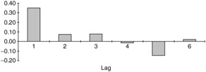
Figure 12.3: A typical correlogram.

We already mentioned that the typical autocorrelation of lag k indicates the relationship between observations k periods apart. The question, however, is how large is a "large" autocorrelation? Under the assumption of randomness, it can be shown that the standard error of any autocorrelation is approximately 1/ , in this case 1/ = 0.1443. (T = 48 which denotes the number of observations in the series.)

EXPONENTIAL SMOOTHING

Dealing with data, many times we are willing to use moving averages to smooth our observations. When we do that, we make our forecast based on equal weight of each value in our observations. Many people would argue that if next month's forecast is to be based on the previous 12 months' observations, then more weight ought to be placed on the more recent observations. The second criticism is that the moving averages method requires a lot of data storage. This is particularly true for companies that routinely make forecasts of hundreds or even thousands of items. If 12-month moving averages are used for 1000 items, then 12,000 values are needed for next month's forecasts. This may or may not be a concern considering today's relatively inexpensive computer storage capabilities. However, it is a concern of availability of data.

Exponential smoothing is a method that addresses both of these criticisms. It bases its forecasts on a weighted average of past observations, with more weight put on the more recent observations, and it requires very little data storage. In addition, it is not difficult for most business people to understand, at least conceptually. Therefore, this method finds widespread use in the business world, particularly when frequent and automatic forecasts of many items are required.

There are many versions of exponential smoothing. The simplest is called, surprisingly enough, simple exponential smoothing. It is relevant when there is no pronounced trend or seasonality in the series. If there is a trend but no seasonality, then Holt's method is applicable . If, in addition, there is seasonality , then Winters' method can be used. This does not exhaust the list of exponential smoothing models ” researchers have invented many other variations ” but these three models will suffice for us.

Simple Exponential Smoothing

Every exponential model has at least one smoothing constant, which is always between zero and one, and a level of the series at time t. The smoothing constant is denoted by ± , and the level of the series L _t . The level value is not observable but can only be estimated. Essentially, it is where we think the series would be at time t if there were no random noise. The simple exponential smoothing method is defined by the following two equations, where F _t+k is the forecast of Y _t+k made at time t:

L _t = ± Y _t + (l - ± ) L _{t -1}

F _t+k = L _t

Even though you usually won't have to substitute into these equations manually, you should understand what they say. The first equation shows how to update the estimate of the level. It is a weighted average of the current observation, Y _t , and the previous level, L _{t -1} ,with respective weights a and 1 - ± . The second equation shows how forecasts are made. It says that the k-period-ahead forecast, F _t+k made of Y _t+k in period t is the most recently estimated level, L _t .

This is the same for any value of k ‰ 1. The idea is that in simple exponential smoothing, we believe that the series is not really going anywhere . So as soon as we estimate where the series ought to be in period t (if it weren't for random noise), we forecast that this is where it will also be in any future period.

The smoothing constant ± is analogous to the span in moving averages. There are two ways to see this. The first way is to rewrite the first equation, using the fact that the forecast error, E _t , made in forecasting Y _t , at time t - 1 is Y _t - F _t = Y _t - L _{t- 1} . A bit of algebra then gives

L _t = L _{t -1} + ± E _t

This says that the next estimate of the level is adjusted from the previous estimate by adding a multiple of the most recent forecast error. This makes sense. If our previous forecast was too high, then E _t is negative, and we adjust the estimate of the level downward. The opposite is true if our previous forecast was too low. However, this equation says that we do not adjust by the entire magnitude of E _t but only by a fraction of it. If ± is small, say ± = .1, then the adjustment is minor; if ± is close to 1, the adjustment is large. So if we want to react quickly to movements in the series, we choose a large ± ; otherwise , we choose a small ± .

Another way to see the effect of ± is to substitute recursively into the equation for L _t . If you are willing to go through some algebra, you can verify that L _t satisfies

L _t = ± Y _t + ± (1 - ± ) Y _{t -1} + ± (1 - ± ) ² Y _t-2 + ± (1- ± ) ³ Y _t-3 + ...

where this sum extends back to the first observation at time t = 1. With this equation we can see how the exponentially smoothed forecast is a weighted average of previous observations. Furthermore, because 1 - ± is less than one, the weights on the Y's decrease from time t backward. Therefore, if ± is close to zero, then 1 - ± is close to 1, and the weights decrease very slowly. In other words, observations from the distant past continue to have a large influence on the next forecast. This means that the graph of the forecasts will be relatively smooth, just as with a large span in the moving averages method. But when ± is close to 1, the weights decrease rapidly , and only very recent observations have much influence on the next forecast. In this case, forecasts react quickly to sudden changes in the series.

What value of ± should we use? There is no universally accepted answer to this question. Some practitioners recommend always using a value around .1 or .2. Others recommend experimenting with different values of alpha until you reach a measure by which the data smoothing is at optimum.

Holt's Model for Trend

The simple exponential smoothing model generally works well if there is no obvious trend in the series. But if there is a trend, then this method consistently lags behind it. For example, if the series is constantly increasing, simple exponential smoothing forecasts will be consistently low. Holt's method rectifies this by dealing with trend explicitly. In addition to the level of the series T _t , Holt's method includes a trend term, T _t and a corresponding smoothing constant ² . The interpretation of T _t , is exactly as before. The interpretation of T _t is that it represents an estimate of the change in the series from one period to the next. The equations for Holt's model are as follows :

1. L _t = ± Y _t + (l - ± )( L _t-1 + T _t-1 )

2. T _t = ² ( L _t - L _{t -1} ) + (l - ² ) T _{t -1}

3. F _t+k = L _t + kT _t

These equations are not as bad as they look. (And don't forget that the computer typically does all of the calculations for you.) Equation 1 says that the updated level is a weighted average of the current observation and the previous level plus the estimated change. Equation 2 says that the updated trend term is a weighted average of the difference between two consecutive levels and the previous trend term. Finally, equation 3 says that the k-period-ahead forecast made in period t is the estimated level plus k times the estimated change per period.

Everything we said about a (alpha) for simple exponential smoothing applies to both a and ² (beta) in Holt's model. The new smoothing constant beta controls how quickly the method reacts to perceived changes in the trend. If beta is small, the method reacts slowly. If it is large, the method reacts more quickly. Of course, there are now two smoothing constants to select. Some practitioners suggest using a small value of a (.1 to .2) and setting ² equal to a. Others suggest using an optimization option (available in most software) to select the "best" smoothing constants.

Winters' Model for Seasonality

So far we have said practically nothing about seasonality. Seasonality is defined as the consistent month-to-month (or quarter-to-quarter) differences that occur each year. For example, there is seasonality in beer sales ” high in the summer months, lower in other months. Toy sales are also seasonal, with a huge peak in the months preceding Christmas. In fact, if you start thinking about time series variables that you are familiar with, the majority of them probably have some degree of seasonality.

How do we know whether there is seasonality in a time series? The easiest way is to check whether a plot of the time series has a regular pattern of ups and downs in particular months or quarters . Although random noise can sometimes obscure such a pattern, the seasonal pattern is usually fairly obvious. (Some time series software packages have special types of graphs for spotting seasonality, but we won't discuss these here.)

There are basically two extrapolation methods for dealing with seasonality. We can either use a model that takes seasonality into account explicitly and forecasts it, or we can first deseasonalize the data, then forecast the deseasonalized data, and finally adjust the forecasts for seasonality. The exponential smoothing model we discuss here, Winters' model, is of the first type. It attacks seasonality directly. Another approach is the deseasonality ” the ratio to moving averages method.

Seasonal models are usually classified as additive or multiplicative. Suppose that we have monthly data, and that the average of the 12 monthly values for a typical year is 150. An additive model finds seasonal indexes, one for each month, that we add to the monthly average, 150, to get a particular month's value. For example, if the index for March is 22, then we expect a typical March value to be 150 + 22 = 172. If the seasonal index for September is -12, then we expect a typical September value to be 150 - 12 = 138. A multiplicative model also finds seasonal indexes, but we multiply the monthly average by these indexes to get a particular month's value. Now if the index for March is 1.3, we expect a typical March value to be 150(1.3) = 195. If the index for September is 0.9, then we expect a typical September value to be 150(0.9) = 135.

Either an additive or a multiplicative model can be used to forecast seasonal data. However, because multiplicative models are somewhat easier to interpret (and have worked well in applications), we will focus on them. Note that the seasonal index in a multiplicative model can be interpreted as a percentage. Using the figures in the previous paragraph as an example, March tends to be 30% above the monthly average, whereas September tends to be 10% below it. Also, the seasonal indexes in a multiplicative model should sum to the number of seasons (12 for monthly data, 4 for quarterly data). Computer packages typically ensure that this happens.

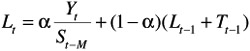
We now turn to Winters' exponential smoothing model. It is very similar to Holt's model ” it again has level and trend terms and corresponding smoothing constants alpha and beta ( ± , ² ), but it also has seasonal indexes and a corresponding smoothing constant ³ (gamma). This new smoothing constant gamma controls how quickly the method reacts to perceived changes in the pattern of seasonality. If gamma is small, the method reacts slowly. If it is large, the method reacts more quickly. As with Holt's model, there are equations for updating the level and trend terms, and there is one extra equation for updating the seasonal indexes. For completeness, we list these equations below, but they are clearly too complex for hand calculation and are best left to the computer. In equation 3, S refers to the multiplicative seasonal index for period t. In equations 1, 3, and 4, M refers to the number of seasons (M = 4 for quarterly data; M = 12 for monthly data). The equations are:

1. 

2. T _t - ² ( L _t - L _{t- 1} ) + (1 - ² ) T _{t -1}

3. 

4. F _t+k = ( L _t + kT _t ) S _t+k-M

To see how the forecasting in equation 4 works, suppose we have observed data through June and want a forecast for the coming September, that is, a 3-month-ahead forecast. (In this case t refers to June and t + k = t + 3 refers to September.) Then we first add three times the current trend term to the current level. This gives a forecast for September that would be appropriate if there were no seasonality. Next, we multiply this forecast by the most recent estimate of September's seasonal index (the one from the previous September) to get the forecast for September. Of course, the computer does all of the arithmetic, but this is basically what it is doing.