VARIABLES DEMONSTRATION TESTS

This section deals with demonstration tests where you can test by variables. Rather than being a straight accept/reject, the variables test will determine whether the product meets other reliability criteria.

FAILURE-TRUNCATED TEST PLANS ” FIXED-SAMPLE TEST USING THE EXPONENTIAL DISTRIBUTION

This test plan is used to demonstrate life characteristics of items whose failure times are exponentially distributed and when the test will be terminated after a pre-assigned number of failures. The method to use is as follows :

First, obtain the specified reliability (R _s ), failure rate ( » _s ), or MTBF ( _s ), and test confidence. Remember that for the exponential distribution:

Then, solve the following equation for various sample sizes and allowable failures:

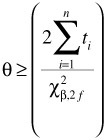
where = MTBF demonstrated; t _i = hours of testing for unit i; f = number of failures; = the ² percentage point of the chi-square distribution for 2f degrees of freedom; and ² = 1 - confidence level.

TIME-TRUNCATED TEST PLANS ” FIXED-SAMPLE TEST USING THE EXPONENTIAL DISTRIBUTION

This type of test plan is used when:

A demonstration test is constrained by time or schedule.
Testing is by variables.
Distribution of failure times is known to be exponential.

The method to use will be the same as with the failure-truncated test. In this case:

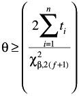
where = MTBF demonstrated; t _i = hours of testing for unit i; f = number of failures; = the ² percentage point of the chi-square distribution for 2(f + 1) degrees of freedom; and ² = 1 - confidence level.

For the time-truncated test, the test is stopped at a specific time and the number of observed failures (f) is determined. Due to the fact that the time at which the next failure would have occurred after the test was stopped is unknown, it will be assumed to occur in the next instant after the test is stopped . This is the reason that the number is added to the number of failures in the degrees of freedom for chi-squared.

How many units must be checked on a 2000- hour test if zero failures are allowed and _s = 32,258? A 75% confidence level is required.

From the information, we know that:

² = 1 - 0.75 = 0.25

2(f + 1) = 2(0 + 1) = 2

Therefore:

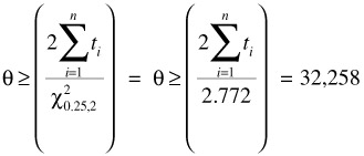
By rearranging this equation, we see that:

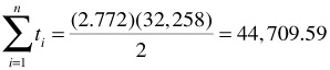
Since no failures are allowed, all units must complete the 2000-hour test and:

= 44, 709.59 = (n)(2, 000)

Solving for n:

n = 44,709.59/2000 = 22.35 or 23 units. We can say that if we place 23 units on test for 2000 hours and have no failures, we can be 75% confident that the MTBF is equal to or greater than 32,258 hours. ( Note: This assumes that the test environment duplicates the use environment such that one hour on test is equal to one hour of actual use.)

Failure-truncated and time-truncated demonstration test plans for the exponential distribution can also be designed in terms of _s , _d , ± , and ² by using methods covered in the sources listed in the references and selected bibliography.

WEIBULL AND NORMAL DISTRIBUTIONS

Fixed-sample tests using the Weibull distribution and for the normal distribution have also been developed. If you are interested in pursuing the tests for either of these distributions, see the sources listed in the selected bibliography.