Chapter 11: Innovation Techniques Used in Design for Six Sigma (DFSS)

MODELING DESIGN ITERATION USING SIGNAL FLOW GRAPHS AS INTRODUCED BY EPPINGER, NUKALA AND WHITNEY (1997)

The signal flow graph represents a diagram of relationships among a number of variables . When these relationships are linear, the graph represents a system of simultaneous linear algebraic equations. The signal flow graph, as shown in Figure 11.1, is composed of a network of directed branches, which connect at the nodes. A branch jk, beginning at node j and terminating at node k, indicates its direction from j to k by an arrowhead on the branch. Each branch jk has associated with it a quantity known as the branch transmission P _jk .

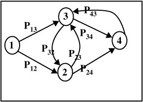
Figure 11.1: A typical branching using signal flow graph.

For our modeling processes, the branches represent the tasks being worked (an activity-on-arc representation). The branch transmissions include the probability and time to execute the task represented by the branch:

P _jk =

where p _jk is the probability associated with the branch; t _jk is the time taken to traverse the branch; and z is the transform variable used to connect the physical system (time domain) to the quantities used in the analysis (transform domain).

The z transform simplifies the algebra, as it enables us to incorporate the quantities to be multiplied (probabilities) in the coefficient of the expression, and to include the quantities to be added (task times) in the exponent. The resulting system is then analogous to a discrete sampled data system, and the body of literature on this subject can be applied for the analysis thereof.

The path transmission is defined as the product of all branch transmissions along a single path. The graph transmission is the sum of the path transmissions of all the possible paths between two given nodes. The graph transmission is also the resulting expression on an arc connecting the two given nodes when all of the other nodes have been absorbed. In particular, we are interested in computing the graph transmission from the start to the finish nodes. Henceforth, graph transmission shall refer to the graph transmission between the start and the finish nodes and is denoted as T _sf .

The coefficient of each term in the graph transmission is the probability associated with the path(s) it represents, and the exponent of z is the duration associated with the path(s). The graph transmission can be derived using the standard operations for the signal flow graphs (discussed below). The impulse response of the graph transmission is then a function representing the probability distribution of the lead time of the process. It can be shown that the expected value of the lead time of the process is:

NUMERICAL EXAMPLE

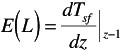
A simple example is shown in Figure 11.2.

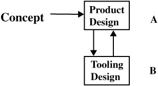
Figure 11.2: A simple example with signal flow graph.

The hypothetical design process is represented by the graph shown in Figure 11.3.

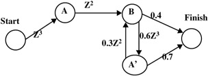
Figure 11.3: A hypothetical design process.

The two tasks A and B (product design and tooling design) take 3 and 2 units of time respectively. Once task B is attempted, task A is reworked with probability 0.6, and once A is attempted, B is reworked with probability 0.3. Iterative repetitions of A are represented by task A'.

The graph transmission is found using the mode elimination technique (discussed below). This graph transmission is given by the equation shown in Figure 11.4.

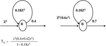
Figure 11.4: The graph transmission.

The expected value of the project lead time E(L) is 7.6 units of time.

The first few terms of the probability distribution function are represented graphically in Figure 11.5.

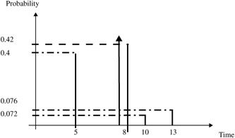
Figure 11.5: First few terms of the probability.

The distribution can be found for this simple example by performing synthetic division on T _sf to obtain the first few terms of the infinite series. The nominal (once through) time for A and B in series is 5 units of time, which occurs with probability 0.4. It is more likely (probability 0.42) that the lead time L of the process will be 8 units of time.

 

RULES AND DEFINITIONS OF SIGNAL FLOW GRAPHS AS INTRODUCED BY HOWARD (1971) AND TRUXAL (1955)

To effectively use signal flow graphs, follow four rules:

1. Signals travel along branches only in the direction of the arrows.

2. A signal traveling along any branch is multiplied by the transmission of that branch.

3. The value of any node variable is the sum of all signals entering the node.

4. The value of any node variable is transmitted on all branches leaving that node.

A path is a continuous succession of branches, traversed in the indicated branch directions. The path transmission is defined as the product of branch transmissions along the path. A loop is a simple closed path, along which no node is encountered more than once per cycle. The loop transmission is defined as the product of the branch transmissions in the loop.

The transmission T of a flow graph is defined as the signal appearing at some designated dependent node per unit of signal originating at a specified source node. Specifically, T _ik is defined as the signal appearing at node k per unit of external signal injected at node j. There are a number of ways of computing transmissions.

BASIC OPERATIONS ON SIGNAL FLOW GRAPHS

Solution of signal flow graphs requires knowledge of certain of their topological properties. The basic operations of addition, multiplication, distribution and factoring can be used to reduce the number of branches and nodes in the system. At first glance, it might appear that by successive application of such transformations a graph could be reduced to a single branch connecting any two given nodes. However, if the graph contains a closed loop of dependencies, as when modeling iterations, one or more self loops will eventually appear.

THE EFFECT OF A SELF LOOP

The effect of a self loop at some node on the transmission through that node is analyzed in Figure 11.6.

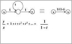
Figure 11.6: The effect of a self loop.

The node signal at the first node is x, and the signal returning around the self loop is xt. Since the node signal is the algebraic sum of the signals entering that node, the external signal arriving from the left must equal y(1 - t). Hence, the effect of a self loop t is to divide an external signal by the factor (1- t) as the signal passes through the node. This holds for all t.

SOLUTION BY NODE ABSORPTION

Node absorption corresponds to the elimination of a variable by substitution in the associated algebraic equations. With the aid of the basic transformations and the self loop replacement, any node in a graph can be absorbed and the equivalent expressions for the transmission between two other nodes calculated. Although the branch is no longer shown, its effects are included in the new branch transmission values, as shown in Figure 11.7.

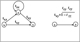
Figure 11.7: Node absorption.

To compute the overall graph transmission, all the intermediate nodes are absorbed in turn , yielding the transmission between the start and finish nodes. Reduction of graphs is computationally intensive , and manual solution of graphs of even moderate size can be difficult.