Visualizing Velocity and Derivative

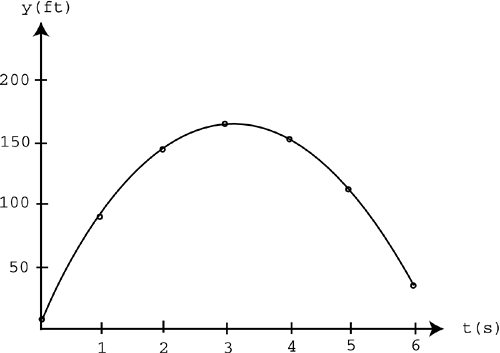
Let's start by revisiting the concept of velocity. Remember that velocity is a vector, so it has direction, and in one dimension that direction is either positive or negative. I also said that average velocity is defined as displacement divided by time. To help visualize the motion of an object, you can start by graphing position versus time on a traditional Cartesian coordinate system. Let's step through the process with a vertical 1D situation like throwing something into the air.

Suppose your game character throws a tomato into the air. You can track the tomato's height as time increases , which gives you the values shown in Table 9.1.

Table 9.1. A Tomato's Height at Various Times

t (in sec )	y (in ft )
	6
1	90
2	142
3	162
4	150
5	106
6	30

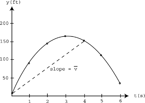
You can then graph these points to see how the tomato moves over time, as shown in Figure 9.1.

Figure 9.1. A graph of the values shown in Table 9.1.

As you can see in the graph, as time increases, the tomato goes up and then falls back down. You can also say that the height ( y ) is a function of time ( t ). That is, the height changes as time increases from 0 to 6 seconds. Mathematically, this can be written as y = f ( t ) and can be read as " y is a function of time." This notation is used throughout the rest of this chapter.

Let's use the graph shown in Figure 9.1 to reexamine the concept of average velocity. Suppose you wanted to know the average velocity of the tomato over the first 4 seconds. If you approached this numerically , you'd have to calculate the displacement and then divide it by the 4-second time interval. Using the new notation, it would look like this:

Average Velocity

= the slope between two points on position v . Time graph for any time interval a t b .

You can also use the graph to visualize this. Remember the good old slope formula? Slope = rise over run. In this case, the rise is the displacement, and the run is the time interval, so the average velocity is simply the slope of the line between those two points on the graph. This is illustrated in Figure 9.2.

Figure 9.2. The average velocity over the first 4 seconds.

Try plugging the coordinates of those two points into the slope formula, and you'll find that you repeated the same process we did earlier. So the slope of the line between any two points on a position-versus-time graph gives you the average velocity over that time interval.

Example 9.1: Finding Average Velocity

Using the data just discussed, find the average velocity of the tomato for the time interval 3 t 5 seconds.

Solution

1. Looking at the data, you need to know the height of the tomato at t = 3s and t = 5s:

   f (3) = 162

   f (5) = 106

2. Calculate the average velocity, or the slope between those two points:

   

   
   

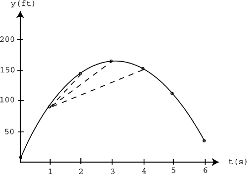
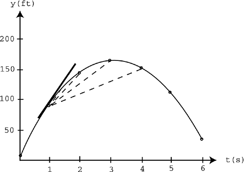
NOTE

If you look at that portion of the graph, you can see that the tomato is falling between 3 and 5 seconds, which is why the average velocity is negative.

At this point, you can calculate the average velocity over any time interval. Let's look at what happens when you take smaller and smaller time intervals. Suppose you want a better understanding of what's happening to the tomato at exactly t = 1s. You can calculate the average velocity between 1 and 4 seconds:

You can calculate the average velocity between 1 and 3 seconds:

You can calculate the average velocity between 1 and 2 seconds:

These smaller and smaller time intervals are illustrated in Figure 9.3.

Figure 9.3. Smaller time intervals close to t = 1.

You can continue to take smaller and smaller time intervals until the line segment approaches a point or an instant in time. This leads to the concept of instantaneous velocity. Look at the dashed lines in Figure 9.3. As the time intervals get smaller and smaller, the dashed lines approach the bold line shown in Figure 9.4. This bold line represents the slope at the point where t = 1s. That slope is the instantaneous velocity at exactly 1 second.

Figure 9.4. Instantaneous velocity at t = 1.

NOTE

The bold line shown in Figure 9.4 is called the tangent line.

The average velocity is the slope of a line segment over a time interval on a position-versus-time graph, and the instantaneous velocity is the slope at a point on the graph. This leads to the concept of the limit. As you take smaller and smaller time intervals, you'll find that the average velocity approaches some number. That is the instantaneous velocity.

Instantaneous Velocity

at t = a for any function f ( t ) that gives position as a function of time.

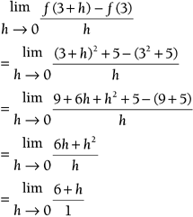
The limit notation might look intimidating, but all it means is keep recalculating the average velocity over smaller and smaller time intervals as close to 0 as you can get.

Example 9.2: Finding Instantaneous Velocity

Suppose you're coding a game like Half Life and the player can throw a grenade into the air, and its height is a function of time, just like the tomato. If its height is y = f ( t ) = t ² + 5, find the instantaneous velocity at t = 3s.

Solution

1. To find the instantaneous velocity at exactly t = 3s, you need to take the average velocity over smaller and smaller time intervals. In other words, take the limit of f ( t ) as the change in time approaches 0:

   

   
   

2. Calculate both heights using the formula y = f ( t ) = t ² + 5:

   

   
   

Here's where the limit notation comes into play. If h keeps getting closer and closer to 0, the instantaneous velocity gets closer and closer to 6.

Believe it or not, you just computed a derivative! A derivative is the rate of change of a quantity as the time interval shrinks to an instant. In this case, you calculated instantaneous velocity , which is the rate of change of height as the time interval approaches 0. The notation for the derivative is the ' (pronounced "prime"). For example, the derivative of f ( t ) is written f '( t ).

Instantaneous Velocity

v = f '( t )

for any position equation that's a function of time, f ( t ).

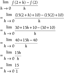
Example 9.3: Finding the Derivative

Suppose a racecar in Need For Speed Under Ground is traveling across the screen, and its position is a function of time defined as y = f ( t ) = 15 t + 10. Find the derivative, or the instantaneous velocity at t = 2s.

Solution

1. To find the instantaneous velocity at exactly t = 2s, you need to find the derivative, or the average velocity as the time interval approaches 0. Use the limit notation:

   

   
   

2. Calculate both positions using the formula y = f ( t ) = 15 t + 10:

   

   
   

3. At this point, it doesn't matter what h is. The derivative is simply 15.

In this section, you computed two derivatives. You used simple polynomial functions (powers of t ) to model the motion of the objects discussed here. However, you could use any function to describe an object's position as time increases. The process is the same; take the limit as the time interval approaches 0, and see what the function approaches. This is only a brief introduction, however. Volumes have been written about tricks and tips for taking the derivative of various functions. If you want to investigate this further, several suggested readings are listed in Appendix B.

Self-Assessment

2.

1.	Looking back at the tomato described in Example 9.1, find its average velocity for the following time intervals: 3 t 6 3 t 5 3 t 4
Looking back at the grenade described in Example 9.2, find its instantaneous velocity at t = 1s.
3.	Suppose an object is thrown into the air, and its height is a function of time. If its height is y = f ( t ) = 3 t 2 + 1, find its instantaneous velocity at t = 5s.
4.	Suppose a vehicle is traveling across the screen, and its position is a function of time defined as y = f ( t ) = 5 t + 2. Find the derivative, or the instantaneous velocity, at t = 3s.