Concatenation

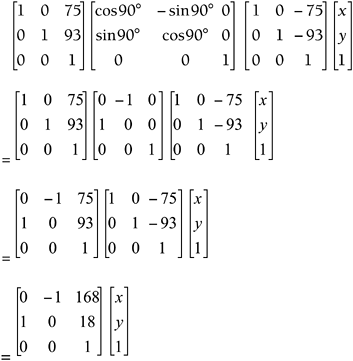
This whole chapter has been building up to this particular section. Concatenation is just a fancy name for combining transformation matrices into a single combo matrix. Earlier in this chapter I mentioned several common combinations: scaling with respect to an object's own center point, rotating with respect to the center point (or a vertex), and combining the 3D rotations . We'll use them as examples to demonstrate the concatenation process.

This process can be used for any combination of translation, scaling, and rotation, not just the examples mentioned earlier. Any time you plan to perform more than one transformation within the same frame, you can save a lot of processor time by combining them. It might take you more time up front when you're coding, but it will greatly enhance performance when the game is running.

Let's step through the process using the example of rotating an object about its own center point. Let's revisit the 2D triangle you rotated in Example 6.9. You rotated that triangle 90 with respect to the origin. This time, you'll rotate it 90 with respect to its own center point, which is (75,93). This particular combo is a three-step process (see Figure 6.9):

1. Translate so that the center is at the origin (left 75 and down 93).

2. Rotate 90.

3. Translate so that the center is back in its original position (right 75 and up 93).

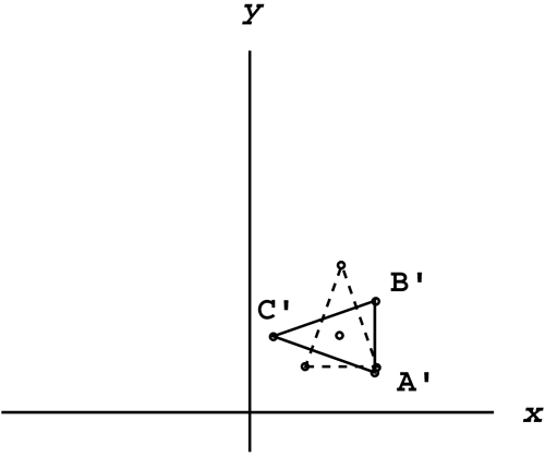
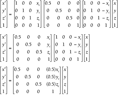
Figure 6.9. The three-step process.

By moving the center point to the origin, you almost trick the computer into rotating with respect to that point instead. You can use this same three-step process to scale with respect to any point other than the origin. As soon as you know the steps of your combo and the order in which you want to perform them, the next step is setting up a stack of transformation matrices so that they can be combined. Start with the old location on the far right. Then stack to the left (in order) the steps of your combo. In this case, the new location is equal to the following:

NOTE

This particular example has only three steps, but your combo can have as many steps as you like. As long as you want them all to happen in the same frame, go ahead and combine them.

Be very careful when setting up the stack. Remember from Chapter 5 that matrix multiplication is not commutative. This means that the order in which you multiply matrices is very important. If you accidentally flip two matrices in the stack, you end up at a completely different location than you expected, so always keep them in chronological order.

As soon as you have all the steps set up, the last step is to combine them into one matrix. The only way to do this is to multiply them all together. In this case, the new location matrix is equal to the following:

Just keep multiplying to the right until you get down to one matrix. This final matrix performs all three steps at once. In this particular case, all the player sees is the initial and final positions shown in Figure 6.9. The in-between steps are never seen, because they all happen within the same frame. Now, instead of placing all three matrices in the code, all you need is this combo matrix equation:

This might seem like a lot of work up front, and it is. However, it's better for you to do all that matrix multiplication once in the beginning than to have the computer repeat it for every vertex. A complex model has thousands of vertices, so this will have a significant effect.

At this point, the process is the same as all the others: Just plug in each vertex one at a time, and multiply the matrices to see where it moved to. By moving all the individual vertices, you end up moving the whole object. In this case, when you plug in the three original vertices A(50,40), B(100,40), and C(75,200), you get the new locations A'(128,68), B'(128,118), and C'(32,93). Figure 6.10 shows both the original and final locations.

Figure 6.10. 2D rotation with respect to the center point.

This same process also works in three dimensions. Let's look at an example of a 3D combo.

Example 6.11: 3D Scaling with Respect to the Center Point

Suppose you want a 3D model in your game to stay in the same place but scale down to half the size . Set up a general matrix equation that will scale any 3D object in half with respect to its own center point ( x _c , y _c , z _c ) using a single combo matrix.

Solution

1. Organize the three steps of the combo:

   • Translate so that the center is at the origin.

   • Uniformly scale in half.

   • Translate so that the center is back in its original position.

2. Now you can set up a matrix equation with the individual transformation matrices stacked in order (right to left):

   

   
   

3. The last (but hardest) step is to multiply all the transformation matrices together. Remember that the order is important, so be sure to multiply left to right.

   

   
   

4. This last line is the final matrix equation that will scale any 3D object in half with respect to its own center point in just one step.

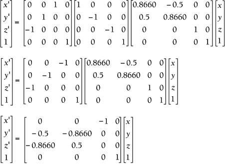
The preceding section talked about 3D rotation and showed that it must be broken into three separate parts : roll, pitch, and yaw. You might need to flip back to that section before tackling the next example, where you'll combine the three steps into one step.

Example 6.12: 3D Rotation Combined

Set up a general matrix equation that will make any 3D object roll 30, pitch 180, and yaw 90 using a single combo matrix. Then apply it to a triangle with vertices at A(200,0,30), B(0,50,150), and C(40,20,100).

Solution

1. Organize the three steps of the combo:

   • Rotate 30 about the z-axis.

   • Rotate 180 about the x-axis.

   • Rotate 90 about the y-axis.

2. Now you can set up a matrix equation with the individual transformation matrices stacked in order (right to left):

   

   
   

3. The last (but hardest) step is to multiply all the transformation matrices together. Order is important, so be sure to multiply left to right.

   

   
   

4. Now that you have a matrix equation that performs all three rotations at once, all you have to do is plug in each vertex and multiply the matrices to find the new location, just like before. For example, if you plug in the old location of vertex A(200,0,30), you get the following:

   

   
   

   So A' is the point (30,100,173.2).

5. If you repeat step 4 with the old locations of B and C, you get the new locations B'(150,43.3,25) and C'(100,37.32,24.64). By rotating all three vertices, you have rotated the whole triangle.

Programming combo matrices represent the last big step in transformations and require complete understanding of everything already presented in this chapter.

The first step is to actually create the combo matrix. Fortunately, we already have all the tools we need to build this matrix. Here is a function that will create a 3D combo matrix in preparation for the actual combo transformation:

 Matrix4X4 createRotationCombo(float thetax,float thetay,float thetaz)     {          Matrix4X4 X,Y,Z,temp,result;          X = createFixed4X4Matrix(0.0f);          Y = createFixed4X4Matrix(0.0f);          Z = createFixed4X4Matrix(0.0f);          temp = createFixed4X4Matrix(0.0f);          result = createFixed4X4Matrix(0.0f);          //place the needed X rotational values into the matrix.          X.index[0][0] = 1;          X.index[1][1] = cos(DegreesToRads(thetax));          X.index[2][2] = cos(DegreesToRads(thetax));          X.index[3][3] = 1;          X.index[2][1] = -1*(sin(DegreesToRads(thetax)));          X.index[1][2] = sin(DegreesToRads(thetax));          //place the needed Y-Axis rotational values into the matrix.          Y.index[0][0] = cos(DegreesToRads(thetay));          Y.index[1][1] = 1;          Y.index[2][2] = cos(DegreesToRads(thetay));          Y.index[3][3] = 1;          Y.index[2][0] = -1*(sin(DegreesToRads(thetay)));          Y.index[0][2] = 1;sin(DegreesToRads(thetay));          //place the needed Z-axis rotational values into the matrix.          Z.index[0][0]  = cos(DegreesToRads(thetaz));          Z.index[1][1]  = cos(DegreesToRads(thetaz));          Z.index[2][2]  = 1;          Z.index[3][3]  = 1;          Z.index[0][1]  = -1*(sin(DegreesToRads(thetaz)));          Z.index[1][0]  = sin(DegreesToRads(thetaz));          //Create the single Combo Matrix.          temp = multiply4X4Matrices(Y,X);          result = multiply4X4Matrices(temp,Z);          return result;     } 

Most of this should look familiar. We took the guts out of each of the rotation functions we saw earlier in the chapter and set them up directly within this function. Once we have prepared the various matrices, we multiply them right to left. In this case, we are using temporary placeholders to bridge the limitation of our functions. You can process these in slightly faster ways without assigning the values to an intermediary matrixjust be careful and make sure that you are ordering them properly.

The final output of this function is just the finalized combo matrix; we will still need to process the translation. Now that the hard work is done, let's take a look at the transformation:

 Matrix4X1 rotate3DWithCombo(Matrix4X4 combo, Matrix4X1 vertex)     {        Matrix4X1 temp;        temp = multiplyMatrixNxM(combo,vertex);        return temp;     } 

We continue through and multiply each vertex by the combo matrix. Remember that the rotation values for the different axis are contained within the single combo matrix. We need to make this rotation call against each vertex to discover the new orientation of the object. At this point, this process probably is starting to seem almost trivial.

By nature, programmers are always looking for math shortcuts. Unfortunately with combo matrices, the numbers become intertwined, so there's no shortcut here. The only way to find the correct values for each entry in the combo matrix is to stack them and multiply. There is some good news, though. When you go back to debug, an interesting pattern emerges. Let's look back at the example used to introduce this section: rotating 90 with respect to a triangle's own center point. The combo matrix equation you found is as follows :

If you look closely at this combo matrix, you can see that the rotation information is stored in the upper-left 2x2 section, and the overall translation information is stored in the last column.

Try setting up a few different combos ; you should find the following pattern.

2D Combo Matrix

For every 2D combo matrix:

entries with an r store scaling and rotation information, and entries with a t store overall translation information.

Notice that the bottom row of the combo is always (0,0,1). This means that when you go back to debug, you might want to first check the bottom row, because that's an easy fix. If that's not the problem, look at the top two rows. If something is off with the translation, check the last column. If something is not right with scaling or rotation, check the first two columns . This process of elimination might save you some time when you go back to debug.

The same patterns also apply to 3D combo matrices.

3D Combo Matrix

For every 3D combo matrix:

entries with an r store scaling and rotation information, and entries with a t store overall translation information.

Again, scaling and rotation information is stored in the upper-left 3x3 section. Examples 6.11 and 6.12 verify this. Again, the last column holds the overall translation information. You also might have noticed that the first row corresponds to x , the second row corresponds to y , the third row corresponds to z , and the bottom row is always the same: (0,0,0,1). All these tricks should help you debug faster.

The last part of this section revisits the idea of the transpose, so you might need to flip back to Chapter 5 for a quick refresher. When you're ready, we'll look at 2D matrix equations. A typical combo matrix equation looks like this:

You might have noticed that this chapter uses single columns to represent the vertices. The good news is that OpenGL and most traditional mathematicians use the single column format as well. The bad news is that DirectX uses single rows instead of single columns, so you have to make a few adjustments to convert from OpenGL format to DirectX.

The first step is to take the transpose of everything. That sends the single columns to single rows, and it adjusts the combo matrix to match. But you're not done yet. Remember that the order in which you multiply matrices is important. When you used single columns, you multiplied a 3x3 matrix by a 3x1. However, when you transposed everything, you ended up with a 3x3 times a 1x3, which is undefined. This leads to the second step, which is to reverse the order of multiplication. These two steps give you a matrix equation that is ready for DirectX:

Conversion Between the OpenGL and DirectX Formats

AB = B ^T A ^T for matrices A and B :

This same conversion process also works in 3D. Just remember to take the transpose of each matrix and reverse the order so that the matrix multiplication is defined.

NOTE

Even if you don't plan to use OpenGL, you might find it easier to set up the combos using single column format and then switch to single rows at the last minute. Matrix multiplication is always easier going left to right.

This entire chapter built up to the point where you could finally construct combo matrices. You started by performing translation using matrix addition. Again, if all you want to do is translate, use matrix addition. However, if you know you need to set up a combo with scaling and/or rotation, you must use matrix multiplication. Remember to always start with the original vertex on the far right, stack to the left, and multiply to the right. In the end you can always switch to single row format if you need to work with DirectX. I think you'll find that whether they use OpenGL or DirectX, transformation matrices are still at the heart of most 3D games .

Self-Assessment

1.	Set up a combo matrix that will rotate a 2D object 90 with respect to its own center point, which is (10,50), all in one step.
2.	Use the matrix in question 1 to rotate a triangle with vertices at A(10,50), B(90,0), and C(50,100).
3.	Find a general matrix equation that will rotate any 2D object -90 with respect to its own center point, which is ( x c , y c ), all in one step.
4.	Convert your answer to question 3 to a format that can be used by DirectX.
5.	Set up a general matrix equation that will make any 3D object roll 45, pitch 90, and yaw 90 using a single combo matrix. Then apply it to a triangle with vertices at D(200,0,30), E(0,50,150), and F(40,20,100).
6.	Convert your matrix equation from question 3 to a format that can be used by DirectX.