6.3. Using an Array Formula

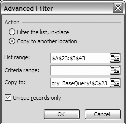
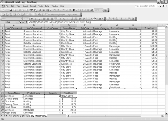
Sometimes you have data that is already partially pivoted. For example, you might have data where you have some descriptive columns and then columns of sales data by year. If you were to use a pivot table to summarize some of the descriptive columns, you would end up having the data by year stacked two data by year rows for each descriptive summary. When some data is stacked, it is often difficult to interpret the information in the pivot table. Even in the examples we used earlier in the chapter with units and quantity, if we summarize both fields with a pivot table, the data ends up stacked, which makes it difficult to interpret the data. If you do not want the data reported this way, you can either write a series of Union queries to un-pivot the data, or you can use the following example.

First, let's start with an example in Excel. Go back to the Excel workbook where we exported the data from the qry_BaseQuery query into an Excel workbook. Assume you want to summarize the data by CenterName and ProductName. The SumIf function does not allow you to use multiple criteria, so you have to find another way to do this. I have worked with a lot of workbooks where someone has needed to do this. They usually sort their data and then perform a SumIf function on multiple subsets of data. While this works, using the same workbook the following month or other reporting period is a challenge.

To avoid this problem, you'll want to use an array formula. It's easiest to show this before explaining it. First, select the two columns of data that you want to summarize, copy them, and paste them starting in cell A23. Then, with that data selected, go to Data Filter Advanced Filter (see Figure 6-6).

Figure 6-6. The Advanced Filter dialog box, which pastes the unique records from a list into a new location

You will be copying the data to a new location using unique records only. Select cell C23 as the new location for your filtered list. You do not need to always place your filtered data beside the data being filtered, but the formulas we're using are dependent on this. Next, delete the list you filtered so you just have a list of unique center names and the products sold at each. To delete the list, use Edit Delete and select "Shift cells left when prompted. This puts the center names in column A and the product names in column B. Using the advanced filter to get unique records is very similar to a group by query from a database. Here is the function to type in cell C24:

     =Sum(IF($D$2:$D$21=A24,IF($G$2:$G$21=B24,$H$2:$H$21,0),0))

Here is the function to type in cell D24:

     =SUM(IF($D$2:$D$21=A24,IF($G$2:$G$21=B24,$I$2:$I$21,0),0))

After you type these formulas in, press Ctrl-Shift-Enter to enter them as an array formula. This uses an IF statement to determine whether the criteria are met. The array formula returns an array of values if you select a multiple cell range and do not use the SUM function. In our case, we just want to return the sum of the array. You may run into situations when you want to nest the IF function further than Excel will let you. In this case, multiply the Boolean results by the range that you want to sum:

     =SUM(($D$2:$D$21=A24) * ($G$2:$G$21=B24)  * ($I$2:$I$21))

Note that in the Excel GUI, FALSE is 0 and TRUE is 1, which is why multiplying the results together works. If any come up false, the result is 0 and the sum doesn't change. Also notice that when you press Ctrl-Shift-Enter, Excel automatically puts braces around the formula, signifying that it is an array formula . Do not attempt to put the braces in yourself, or Excel will give you an error message. Figure 6-7 shows what the resulting worksheet looks like with the IF statement method.

Figure 6-7. The Array formula example, showing what it looks like when you edit the formula

While you can accomplish the same result by using a Group By query in Access, sometimes you want the results to update if the data is changed in Excel, say by a curious user without permissions to reach the original data.

To accomplish this by automation from Access, use the approach in Example 6-6.

Example 6-6. Array formula example

 Public Sub ArrayFormulaExample(  ) Dim xlapp As Excel.Application Dim xlwb As Excel.Workbook Dim xlws As Excel.Worksheet Dim xlrng As Excel.Range Dim adors As ADODB.Recordset Dim adofld As ADODB.Field Dim w, x, y, z As Integer Set xlapp = New Excel.Application xlapp.Visible = True Set xlwb = xlapp.Workbooks.Add Set xlws = xlwb.ActiveSheet xlws.Name = "BaseData" Set adors = New ADODB.Recordset adors.Open "qry_BaseQuery", CurrentProject.Connection, adOpenStatic, adLockReadOnly x = 1 For Each adofld In adors.Fields   xlws.Cells(1, x).Value = adofld.Name   x = x + 1 Next adofld Set xlrng = xlws.Cells(2, 1) xlrng.CopyFromRecordset adors y = adors.RecordCount + 1 adors.Close Set xlrng = xlws.Cells(y + 2, 1) xlrng.Value = "Center Name" Set xlrng = xlws.Cells(y + 2, 2) xlrng.Value = "Product Name" Set xlrng = xlws.Cells(y + 2, 3) xlrng.Value = "Quantity" Set xlrng = xlws.Cells(y + 2, 4) xlrng.Value = "Cost" Set xlrng = xlws.Cells(y + 3, 1) adors.Open "Select CenterName, ProductName from qry_BaseQuery " & _        "Group by CenterName, ProductName", CurrentProject.Connection, _        adOpenStatic, adLockReadOnly xlrng.CopyFromRecordset adors w = y + 2 + adors.RecordCount For z = (y + 3) To w   Set xlrng = xlws.Cells(z, 3)   xlrng.FormulaArray = _   "=SUM( (RC1=R2C4:R" & y & "C4) * (RC2=R2C7:R" & y & "C7) * " & _   "(R2C8:R" & y & "C8))"   Set xlrng = xlws.Cells(z, 4)   xlrng.FormulaArray = _   "=SUM( (RC1=R2C4:R" & y & "C4) * (RC2=R2C7:R" & y & "C7) * " & _   "(R2C9:R" & y & "C9))"   xlrng.Style = "Currency" Next z xlws.Columns.AutoFit adors.Close Set adofld = Nothing Set adors = Nothing Set xlrng = Nothing Set xlws = Nothing Set xlwb = Nothing Set xlapp = Nothing End Sub

This method also can be used when you want to get pivot table-like results that update automatically, instead of when the user presses "Refresh data." Another way this method can be used is to multiply the Boolean results together using the SUM function, simulating the CountIf function but allowing you to use multiple criteria.