5.6 Channel Capacity Calculation

The channel capacity for the indoor radio frequency environment can be calculated based on the received signal strength and the corresponding noise level. The received signal strength depends on the transmit signal power level and the indoor radio frequency channel loss. According to the FCC rule, 1 W of transmit power is allowed at a spectrum of 1 MHz. This translates to a power spectrum density level of -30 dBm/Hz. On the other hand, the FCC rule clearly states that the transmit power spectrum density is limited at -32 dBm/Hz in every 3-kHz bandwidth. According to Figures 5.11 and 5.12, the worst case channel losses are 70 and 78 dB at less than 30 ft for frequency bands of 2.4 and 5.7 GHz, respectively. The channel capacity can be calculated according to

Equation 5.58

The answer is expressed in terms of bits per hertz. Assuming a noise power spectrum density of -168 dBm/Hz. The channel capacity for the 2.4-GHz frequency band is shown by

Equation 5.59

corresponding to the signal power spectrum density of -32 - 70 = -102 dBm/Hz. For the same noise power spectrum density level, the channel capacity for the 5.7-GHz frequency band is shown by

Equation 5.60

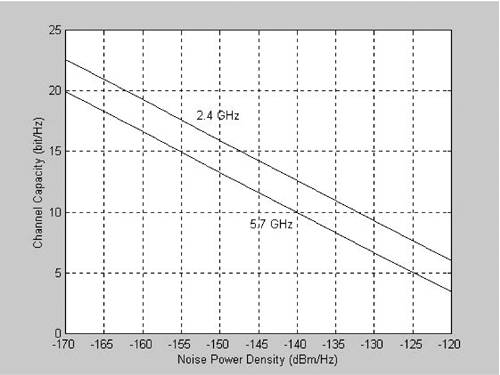
corresponding to the signal power spectrum density of -32 - 78 = -110 dBm/Hz. These calculations are based on a radio frequency interference-free environment where the noise floor is determined by the environment thermal noise. However, this indoor radio frequency channel is within an IMS band and the channel might be contaminated by radio frequency interference noise from other IMS band transmission systems. Figure 5.20 shows channel capacity figures corresponding to different noise power spectrum density levels for 2.4- and 5.7-GHz frequency bands, respectively. For a signaling bandwidth of 1 MHz, a channel capacity of 12 bits/Hz, which can be maintained with a noise power spectrum density level of -150 dBm/Hz, can be designed for a transmission system with a throughput of 10 Mbps. Figure 5.20 indicates that some research and study activities can be conducted for the development of high throughput, 10 Mbps and above, indoor radio frequency transmission systems.

Figure 5.20. Channel Capacity versus Noise Power Density

graphics/05fig20.jpg

5.7 MATLAB/Simulink Models

5.7.1 Reflection Coefficient

[View full width]


[View full width]

%clear
m1=1;
m2=1;
e1=1;
e2=9;
n1=sqrt(m1/e1);
n2=sqrt(m2/e2);
thtaid=[0:90];
thtai=thtaid/180*pi;
thtar=thtai;
thtat=acos(cos(thtai).*sqrt(m1*e1/m2/e2));
ii=1;
for i=1:91
   if imag(thtat(i))~=0
      ii=ii+1;
   end
end
whitebg('white')
figure(1)
plot(thtaid,thtat/pi*180,'k')
grid
xlabel('Incident Angle (Degree)')
ylabel('Transmit Angle (Degree)')
R1=ones(91,1);
R2=ones(91,1);
T1=zeros(91,1);
T2=zeros(91,1);
R1(ii:91)=((-n1.*sin(thtai(ii:91))+n2.*sin(thtat(ii:91)))./(n1.*sin(thtai(ii:91))+n2.*sin

(thtat(ii:91)))).^2;
R2(ii:91)=((n2.*sin(thtai(ii:91))-n1.*sin(thtat(ii:91)))./(n2.*sin(thtai(ii:91))+n1.*sin

(thtat(ii:91)))).^2;
T1(ii:91)=(4*n1*n2.*sin(thtai(ii:91)).*sin(thtat(ii:91)))./(n1.*sin(thtai(ii:91))+n2.*sin

(thtat(ii:91))).^2;
T2(ii:91)=(4*n1*n2.*sin(thtai(ii:91)).*sin(thtat(ii:91)))./(n2.*sin(thtai(ii:91))+n1.*sin

(thtat(ii:91))).^2;
whitebg('white')
figure(2)
plot(thtaid,R1,'k',thtaid,T1,'k');
grid
xlabel('Angle (Degree)');
ylabel('Coefficient');
gtext('Parallel Reflection Coefficient')
gtext('Parallel Transmit Coefficient')
whitebg('white')
figure(3)
plot(thtaid,R2,'k',thtaid,T2,'k');
grid
xlabel('Angle (Degree)');
ylabel('Coefficient');
gtext('Perpendicular Reflection Coefficient')
gtext('Perpendicular Transmit Coefficient')

5.7.2 Signal Strength

d=[3:50];
l1=0.32*39.37/12;
l2=0.12*39.37/12;
l3=0.052*39.37/12;
lu=0.5;
ll=3;
data1=[3.5 6; 3.5 14; 3.9 12; 5 11; 5 19; 5 24; 7 15; 7.3 13; 7.3 17; 
7.3 24; 7.3 27; 7.5 20; 7.5 18; 8.2 21; 8.2 27; 9.0 18; 9.0 28; 9.0 30; 
10 20; 10 26; 12 32; 12 35];
data2=[2.3 6; 2.3 12; 3.1 7; 3.1 11; 3.5 13; 4 12; 4 19; 4 24; 5 8;
5 12; 5 15; 5 21; 6 20; 7 16; 7 29; 8 22; 8 32; 9 25; 9 28; 10 24;
10 30; 13 23; 13 26; 13 27; 13 33; 13 39];
whitebg('white')
figure(1)
provptu=10*log10(l1^2/16/pi^2/lu./d.^2);
provpt=10*log10(l1^2/16/pi^2./d.^2);
provptl=10*log10(l1^2/16/pi^2/ll./d.^2);
plot(d,provptu,'k',d,provpt,'k',d,provptl,'k');
grid
xlabel('Distance (ft)')
ylabel('Attenuation (dB)')
whitebg('white')
figure(2)
provptu=10*log10(l2^2/16/pi^2/lu./d.^2);
provpt=10*log10(l2^2/16/pi^2./d.^2);
provptl=10*log10(l2^2/16/pi^2/ll./d.^2);
plot(d,provptu,'k',d,provpt,'k',d,provptl,'k',data1(:,1)*39.37/12,-data1(:,2)-40,'kx');
grid
xlabel('Distance (ft)')
ylabel('Attenuation (dB)')
whitebg('white')
figure(3)
provptu=10*log10(l3^2/16/pi^2/lu./d.^2);
provpt=10*log10(l3^2/16/pi^2./d.^2);
provptl=10*log10(l3^2/16/pi^2/ll./d.^2);
plot(d,provptu,'k',d,provpt,'k',d,provptl,'k',data2(:,1)*39.37/12,-data2(:,2)-46,'kx');
grid
xlabel('Distance (ft)')
ylabel('Attenuation (dB)')

5.7.3 Channel Impulse Response Model

for j=1:20
   ModelType='OBS';
%Separation distance Eexpressed in meet
Dn=5;
switch ModelType
   % For line-of-sight
case 'LOS'
% Probability of receiving a multipath
for i=1:14
   PTk(i)=1-i*7.8/367;
end
for i=15:25
   PTk(i)=0.65-(i*7.8-110)/360;
end
for i=26:64
   PTk(i)=0.22-(i*7.8-200)/1360;
      end
      % Delay related path loss exponent
      for i=1:2
   nTk(i)=2.5+i*7.8/39;
end
for i=3:32
   nTk(i)=3+(i*7.8-15.6)/380;
end
for i=33:64
   nTk(i)=3.6;
      end
      % Mean
      mean1=10*nTk*log10(Dn/2.3);
      % Standard Deviation
std1=4;
   case 'OBS'
% Probability of receiving a multipath
for i=1:12
   PTk(i)=0.55+i*7.8/667;
end
for i=13:64
   PTk(i)=0.08+0.62*exp(-(i*7.8-100)/75);
end
      % Delay related path loss exponent
      for i=1:39
   nTk(i)=3.65+i*7.8/536;
end
for i=40:64
   nTk(i)=4.23;
end
      % Mean
      mean1=10*nTk*log10(Dn/2.3);
      % Standard Deviation
      std1=5;
   otherwise
end
OcTk=ceil(PTk-rand(1,64));
Ak1=zeros(1,64);
Ak0=rand(1,64)*std1+mean1;
for i=1:64
   if OcTk(i)==1
      Ak1(i)=Ak0(i);
   end
end
ak1=zeros(1,64);
for i=1:64
   if OcTk(i)==1
      ak1(i)=10^(-Ak1(i)/20);
   end
end
plot([1:64],ak1/max(ak1),'k')
aak1(j,:)=ak1;
end
mesh(aak1/max(aak1(:,1)))
view(30,30)
xlabel('Excess Delay (ns)')
ylabel('Channel Index')
zlabel('Relative Magnitude')

5.7.4 Baseband Channel Model

ModelType='LOS';
%Separation distance Eexpressed in meet
Dn=5;
switch ModelType
   % For line-of-sight
case 'LOS'
% Probability of receiving a multipath
for i=1:14
   PTk(i)=1-i*7.8/367;
end
for i=15:25
   PTk(i)=0.65-(i*7.8-110)/360;
end
for i=26:64
   PTk(i)=0.22-(i*7.8-200)/1360;
      end
      % Delay related path loss exponent
      for i=1:2
   nTk(i)=2.5+i*7.8/39;
end
for i=3:32
   nTk(i)=3+(i*7.8-15.6)/380;
end
for i=33:64
   nTk(i)=3.6;
      end
      % Mean
      mean1=10*nTk*log10(Dn/2.3);
      % Standard Deviation
std1=4;
   case 'OBS'
% Probability of receiving a multipath
for i=1:12
   PTk(i)=0.55+i*7.8/667;
end
for i=13:64
   PTk(i)=0.08+0.62*exp(-(i*7.8-100)/75);
end
      % Delay related path loss exponent
      for i=1:39
   nTk(i)=3.65+i*7.8/536;
end
for i=40:64
   nTk(i)=4.23;
end
      % Mean
      mean1=10*nTk*log10(Dn/2.3);
      % Standard Deviation
      std1=5;
   otherwise
end
OcTk=ceil(PTk-rand(1,64));
Ak1=zeros(1,64);
Ak0=rand(1,64)*std1+mean1;
for i=1:64
   if OcTk(i)==1
      Ak1(i)=Ak0(i);
   end
end
ak1=zeros(1,64);
for i=1:64
   if OcTk(i)==1
      ak1(i)=10^(-Ak1(i)/20);
   end
end
figure(1)
plot([1:64],ak1/max(ak1),'k')
xlabel('Excess Delay (ns)')
ylabel('Channel Index')
%raised cosie pulse
alp=0.15;
xt=[-385:385]/64;
gt=sin(pi*xt)./(pi.*xt).*cos(alp.*pi.*xt)./(1-(2.*alp.*xt).^2);
gt(386)=1;
figure(2)
plot(xt,gt)
gtchnl=zeros(1,834);
for i=1:64
   gtchnl(i:i+770)=ak1(i).*cos(2*pi*2.4e9*(i-1)*7.8e-9)*gt+gtchnl(i:i+770);
end
figure(3)
plot(gtchnl)
maxgtchnl=max(gtchnl);
mingtchnl=min(gtchnl);
if maxgtchnl>-mingtchnl
   gtchnl=gtchnl/maxgtchnl;
else
   gtchnl=gtchnl/mingtchnl;
end
for i=1:834
   if gtchnl(i)==1;
      maxj=i;
   end
end
xtgtchnl=([1:834]-maxj)/64;
figure(4)
plot(xt,gt,'k',xtgtchnl,gtchnl,'k')
grid
xlabel('Symbol Interval')
ylabel('Magnitude')

Flylib.com

Category list

Similar pages

5.6 Channel Capacity Calculation