4.2 In-House Electrical Wiring Model

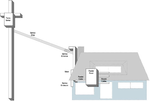
Electricity has found its applications in every household for about 100 years. To ensure the safe use of electricity, the first edition of the National Electrical Code (NEC) was published during 1897. Since then the NEC has been updated every two or three years to keep up with technological developments [2]. The National Fire Protection Association has acted as a sponsor for the NEC since the 1911 edition. NEC gives guidelines on methods, material, wiring, and protection for residential and other end-user applications. The essential part of the NEC has been voluntarily adopted by most states and municipalities. NEC has provided safety for electricity usage and uniformity in wiring practices.

4.2.1 Wiring Practice

An average residential unit is connected to the distribution transformer through a service drop as shown in Figure 4.10. A service drop usually has three conductors: two each for 120 V of opposite phases (for a combined 240 V) and one for a neutral. Starting from the service entrance, service cables go through a usage meter and are terminated at the service enclosure box. Feeder cables are then used to connect the service enclosure box and the feeder panel.

Figure 4.10. Distribution Structure

Branch cables are used to connect lights and appliances to the feeder panel. A feeder panel can have a few dozen branch cables all individually protected by circuit breakers as shown in Figure 4.11. A ground is also created for each unit by inserting an electrode deep into the soil. The ground is bonded to the neutral at the feeder panel. Any branch cable can include the ground wire for leakage protection. The ground wire can be connected to metal enclosures of appliances. Any leakage on the metal enclosure will then go through the ground wire to neutral forming a short circuit and causing the circuit breaker to break.

Figure 4.11. Feeder Panel

A circuit breaker and associated branch cable are usually dedicated to a particular room or area within a household as shown in Figure 4.12. Sometimes multiple branches might be required for a certain area. For example, the kitchen area might have a branch for all the lights, a branch for appliances, and another branch of 240 V for an electrical range. An interlocked two-phase circuit breaker is used for a 240-V branch cable with three conductors. Otherwise, two phases of electrical supplies are randomly used for different branches of 120 V to equalize the load. Sometimes, electrical outlets on different walls of the same room can come from different phases.

Figure 4.12. In-House Wiring Configuration

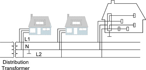
Depending on its dimension, the length of a branch cable can be as long as the sum of the depth, width, and height of a house. A single-storey house of 800 square feet might, for example, have a depth of 26 feet, a width of 30 feet, and a height of 9 feet. An average-size two-storey home can be 28 feet deep, 38 feet wide, and 18 feet high while a large home of 3800 square feet can have a depth of 30 feet, a width of 40 feet, and a height of 20 feet plus a walk-up attic. Therefore the longest branch in a house can range from 65 to 90 feet. Another important factor is that a distribution transformer is shared among a number of households as shown in Figure 4.13. In North America, a transformer is usually shared by five households. The number of households can be increased to 25 in certain areas. Because of this shared nature, an in-home electrical wiring based transmission system might interfere with an similar system of your neighbors. A Media Access and Control protocol layer should be properly designed to avoid such an interference. Furthermore, some encryption and authentication measures should also be considered for privacy issues.

Figure 4.13. General Distribution Structure

4.2.2 Lights and Appliances as Terminals

When electrical devices are turned off, impedances of these devices are not attached to branch cables. Terminals of branch cables can be considered open ended except that some capacitors can still be attached for surge protection. These capacitors can have a capacitance of up to a few microfarads. When a light is on, its load resistance can be calculated according to its power rating. For example, a 60 W, 120-V light bulb allows a current of 0.5 amperes and, therefore, has a load resistance of 240 ohms. On the other hand, a heavy-duty appliance consuming a few kilowatts has a much smaller load resistance. For example, a 3600 W, 240-V oven allows a current of 15 amperes and has a load resistance of only 16 ohms. Most electrical loads are resistive, such as lights, or partially inductive, such as motors or voltage converting power supplies in appliances.

Depending on the time of the day and activities, the electrical load within a household is dynamic, which means that the total load resistance changes from time to time on the usage time scale of a few minutes by human intervention. On the other hand, many electrical devices with automatic control, such as a refrigerator or an air conditioner, can vary their load resistance on a time scale of a few seconds. Furthermore, some devices such as a light dimmer or a motor speed controller can turn on and off an electrical device in a fraction of a second. An electronic dimmer switch uses a transistor-like device called a TRIAC to switch the electricity on and off 120 times each second. One cycle of household 60 Hz AC electrical power is shown in Figure 4.14. A TRIAC turns itself off each time voltage reverses direction/sign/polarity and then on after a certain delay. The rotating or sliding control on the switch decides the delay time. As the delay time becomes shorter, the light is on more of the time and is, thus, brighter. As the delay time goes longer, the light is on less of the time and is, thus, dimmer.

Figure 4.14. The Operation of a Dimmer Switch

Load terminations on electrical wiring are very dynamic. They can be at the middle or end of a branch cable. We call a load termination in the middle of a branch cable a bridged load termination. Load terminations can also be attached and detached from time to time. Even when attached, they can be switched on and off rapidly. As far as using the electrical wiring as a transmission medium is concerned, the open-ended, bridged, as well as low-impedance terminations can all cause significant reflections. Another important factor is that branch cables are generally imbalanced despite the parallel construction of the cable as far as the radio emission is concerned. This is in part because light switches are often used to break only the hot but not the neutral conductor. Cable imbalance can also be caused by the wiring of three-way light switches.

4.2.3 Channel Models

A channel model of in-house power lines can be constructed based on a model wiring configuration, cable model, and two-phase crosstalk model. Figure 4.15 shows a simple wiring configuration with four one-phase branches on each phase and one two-phase branch across phases. This simplified configuration model is used as an illustration. Many real wiring configurations can have more than a dozen one-phase branches on each phase and a few two-phase branches.

Figure 4.15. A Typical Wiring Configuration

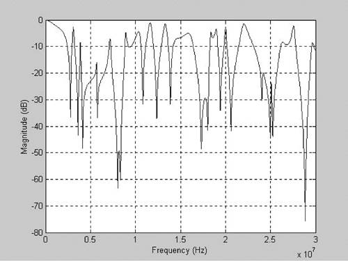
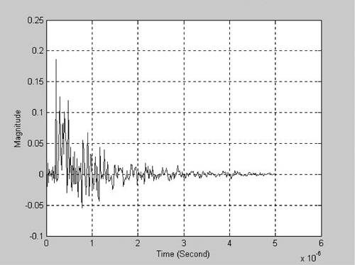
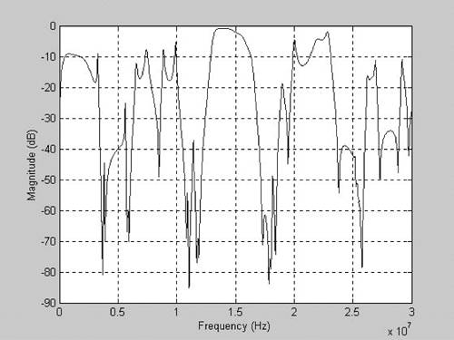
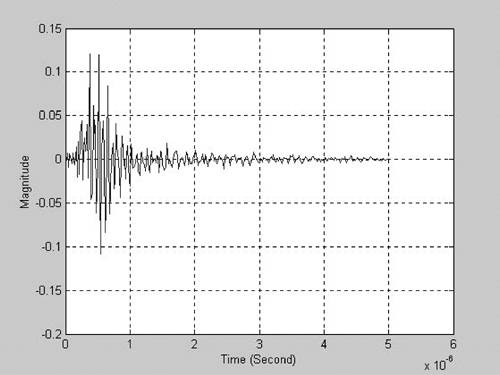
We first construct a channel model within the same phase of this wiring model. This one-phase channel model starts at point A and ends at point B. Only effects of other branches of the same phase are included, and the effects of the other phase is omitted. Figure 4.16 shows the transfer function of this simple one-phase in-house power line channel model. While the minimum attenuation is not bad, many notches of 40 to 50 dB can be observed. The average attenuation can become heavier if some branches are terminated with lights or appliances or more branches are present. In time domain, Figure 4.17 shows the impulse response of this simple one-phase in-house power line channel model. The delay spread is about 4 µsec.

Figure 4.16. Frequency Response from Point A and Point B

Figure 4.17. Impulse Response from Point A to Point B

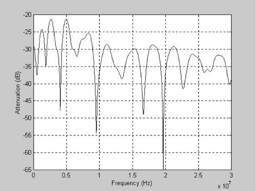
We then consider a channel model across two different phases of this wiring model. This two-phase channel model starts at point A and ends at point C. Effects of all branches connected on two phases as well as the crosstalk within a three-conductor cable are considered. In this example, the coupling effect of the three-conductor cable is the main transmission mechanism across two phases. Figure 4.18 shows the transfer function of this simple two-phase in-house power line channel mode. Attenuations are heavier in general because of the effect of crosstalk attenuation between two phases of the three-conductor branch. Notches become deeper and wider because of the increased number of branches. This two-phase channel model can also become much worse if some branches are terminated with lights or appliances or more branches are present.

Figure 4.18. Frequency Response from Point B to Point C

Again in time domain, Figure 4.19 shows the impulse response of this simple two-phase in-house power line channel model. Alternatively we can generate random channel models and select those that closely resemble field measurements. A generic random in-house power line channel model has been suggested by researchers at the University of Karlsruhe [6]. This random channel model can be expressed by

Equation 4.30

Figure 4.19. Impulse Response from Point B to Point C

This model consists of N transmission or reflection paths. Parameters a₀, a₁, and k correlate to the type of cable used in the in-house power line wiring. d_i determines the length of each path. controls the magnitude of the transmitted or reflected signal and regulates corresponding phases, where v_p = 150 x 10⁶ meters per second (m/sec) is the speed of propagation. With this approach, a wiring configuration is not required. In fact, sometimes an accurate wiring configuration is difficult to obtain. With some considerations on choices of a₀, a₁, and k based on cable type and experimental experience, we can let a computer generate random models and pick a few that satisfy our objectives. For an example, we can set the maximum length of each branch at 150 and let g_i be a random number between 0.1 and 0.1. Figure 4.20 shows the transfer function of a particular channel model of 100 different random samples. In this simulation, we have used a₀ = 0, a₁ = 8 x 10 ⁶, k = 0.5, and N = 10. Figure 4.21 shows the corresponding impulse response. We only observed a few strong reflections. Better models might be discovered by running many more simulations.

Figure 4.20. A Computer-Generated In-House Wiring Model

Figure 4.21. Corresponding Impulse Response