Lesson 1: Moving from OLAP Data Warehouses to Cubes

Previous chapters illustrated that the basic process of building a data warehouse and OLAP system is started by performing the following steps:

• Determine requirements.
• Design and build the data warehouse database.
• Extract and load data.

After these steps have been performed, the final step is designing and building the OLAP cubes. The level of success in designing and building the OLAP cubes is determined by how well these preceding steps have been carried out.

After this lesson, you will be able to:

• Describe online analytical processing (OLAP)
• Describe a data cube
• Understand the relationship between the structure of your data warehouse and the cubes you will build
• Recognize the most important data warehouse design elements
• Differentiate between the data warehouse and multidimensional analysis structures

Estimated lesson time: 40 minutes

Determining Requirements

The best hardware and software will not bring success if the requirements of the data warehouse have not been as thoroughly determined as possible. Two ironies make this aspect of building a data warehouse particularly challenging:

• The full set of requirements will not usually be completely understood until the data warehouse has been constructed.
• Even the same types of businesses will not likely have the same requirements for their data warehouses because different businesses will value different measurements of success or key performance indicators.

Business and User Requirements

The first step in building a data warehouse and OLAP system is careful analysis of the business and user needs. A warehouse may have a wealth of aggregations, but if the dimensions do not reflect the business structure, the data will be difficult to use.

Technical Requirements

These business requirements must be evaluated in conjunction with the technical requirements. For example, if the storage space required for a given level of granularity is in the multi-terabyte range, the cost of storage may be prohibitive. You would then need to adjust your design accordingly by selecting a higher level of granularity, adjusting the lifetime of warehoused data, or perhaps both.

Designing and Building the OLAP Data Warehouse Database

There are several steps to follow in order to create an OLAP database. The OLAP database is the basis for the cubes that you build with OLAP Services. Determining the fact and dimension tables lays the groundwork for building dimensions and data cubes.

Design the Database

When designing a database,

• Use a denormalized database design to support typical data warehouse queries
• Use a star schema

Once the database has been designed, the database, tables, and indexes are created.

Create the Tables

One of your most important tasks is to identify the fact and dimension tables.

• Fact tables represent the data on which you want to report.

If your main business is selling a product, you will want to know how many of each product you sell.

• Dimension tables break up the data according to a variety of criteria, called dimensions.

For example, you may want to know how many of each product you sell by region of the country (location dimension) and how many you sell in a particular quarter, month, or day (time dimension).

Create the Indexes

Indexes speed data access for regular queries and are used by OLAP Services when it builds cubes based on the underlying fact tables. Because the warehouse provides users with read-only access, you can create a number of indexes to speed up retrievals without concern for impact on inserts and updates. It is important to identify the primary queries that the users will perform and index along the dimensions of those queries. The SQL Server Index Tuning wizard can assist in this process.

Extracting, Cleaning, and Loading Data

Once the database has been created, the data must be loaded from the OLTP systems into the data warehouse. SQL Server 7.0 provides an application called Data Transformation Services (DTS) that allows data to be moved from various data sources into the data warehouse. During this period you can perform several steps:

• Data validation

Validation ensures that the data is correct at the source before it is migrated to the warehouse. If you migrate incorrect data and correct it in the warehouse, the source data will still be incorrect.

• Data migration

Migration is moving the data from the source, either directly to the target or into an intermediate database. If the data is migrated to an intermediate database, this is where data scrubbing occurs.

• Data scrubbing

Scrubbing is the process of making the data consistent. For example, if you pull data from a site in Canada and from a site in Germany, sales in the two databases may have been recorded in the local currencies. Scrubbing will convert the sales to a common currency so the data is consistent in the warehouse.

• Data transformation

Transformation is the process of changing data before it is placed in the warehouse. For example, a particular field may need to be broken up into several separate fields, or several fields may need to be combined into one field. It is possible to pre-aggregate data during this step.

After these processes are performed, the data is moved into the warehouse. You can now build OLAP cubes based on the underlying data warehousing tables.

Figure 9.1 shows the Northwind_Mart database OLAP star schema. The Sales_Fact table has measures in it. A measure is any quantifiable datum that the data warehouse should measure: dollars in an order, quantity shipped, or orders taken by an employee, for example. Any metric that provides valuable information about business operations is a valid measure, provided that information can be captured from operational systems. These measures are the values that end users want to see in dimensional analysis.

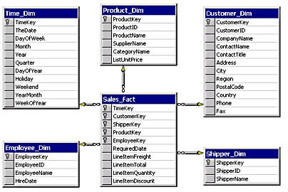
Figure 9.1 Northwind_Mart OLAP Star Schema

The other tables are the dimension tables that represent how users will view the measures in other words, how the data is to be filtered and subdivided. For example, you may want to see orders taken by a particular employee (filter), for each quarter over the past two years (subdivision, also known as dimension levels).

Multidimensional Structure (Cube)

The following is a very simple example of a cube.

You are the owner of a coffee stand. You have two employees, Claire and William. In order to pay each appropriately for their hard work, you track which employee sells how much of each item sold daily.

	Col A	Col B	Col C
Row 1	Friday	Claire	William
Row 2	Regular	20	15
Row 3	Decaf	18	11
	Col A	Col B	Col C
Row 1	Saturday	Claire	William
Row 2	Regular	30	22
Row 3	Decaf	22	19
	Col A	Col B	Col C
Row 1	Sunday	Claire	William
Row 2	Regular	18	12
Row 3	Decaf	18	11

If you were to stack these reports on a corner of your desk, you would create a multidimensional cube. If you wanted to analyze Claire s sales, you could "slice" your stack of reports down Column B. If you wanted to analyze how well decaf sells, you would "slice" along Row 3.

This is admittedly an extremely simple example. However, even the most complex multidimensional analysis is merely a computer-based extension of this simple process. Thankfully, computers find it much easier than most humans to think in multidimensional terms.

Data cubes are multidimensional structures that store the data for your OLAP system. Multidimensional means that cubes allow you to look at your data in various ways. In Figure 9.2, you want to know product sales by region and by time. The three dimensions are

• Product
• Location
• Region

Figure 9.2 Graphical representation of a cube

Each cell holds one value, exactly as a spreadsheet does. The address or location of each cell is the intersection of each dimension. The data or value in the cell is a summarized number from the online transaction processing (OLTP) system.

The cube holds the sales for all your products in the various locations, by period. To get an annual total, choose a product and location, and sum up the four period cells to get annual sales by product and location.

Alternatively, you could create a second cube that has all products by all locations, where the time slice is just an annual total. The cube will then be smaller, but you will no longer be able to retrieve totals by period you will be able to retrieve only annual totals. This is where careful analysis will reveal the needs of the system and determine the cost of adding cubes as compared with the required response times.

For each dimension in a cube, you define a hierarchy by the data to access. For example, location might actually be a hierarchy in which

• Locations are subdivided into territories
• Territories are subdivided into markets
• Each market consists of a number of individual stores

With this structure, you can start at a location and drill down to a specific store.

Lesson Summary

This lesson emphasized how important and interdependent are data warehouse design decisions. For example, dimension and fact tables can be designed only after sufficient analysis and user interviews. The cubes that these end users will consume are wholly dependent on the denormalized data warehouse database.