| This section shows how to program in Sling. Playing with Sling is fun. You can start the Sling IDE with > java sjm.examples.sling.SlingIde 16.3.1 A Basic Sling Sling lets you plot mathematical functions by issuing plot commands. The namesake of Sling is the sling() function, which takes two arguments: the length of the sling strap, and the number of times the sling goes around (one's head). For example, to plot the path of a sling whose strap length is 1 and that travels three- quarters of a revolution, run the class SlingIde and enter the Sling program plot sling(1, .75); Click the Go! button in the IDE or press the Ctrl and G keyboard keys to make the program execute. Figure 16.1 shows the results. Figure 16.1. A basic sling. This plot shows the path of sling, seen from overhead. This sling has a strap length of 1 and circles the hurler's head 0.75 times.  You can plot a complete circle by setting the second argument to the sling function to 1 : plot sling(1, 1); // a complete circle You can also specify a number greater than 1 for the number of revolutions and still get a circle: plot sling(1, 3); // still a circle A sling that goes around three times traces the same circle three times. 16.3.2 Adding Slings To make the plot more interesting, you can attach a second, smaller sling to the end of the first sling using the command plot sling(1, 1) + sling(.5, 5); Figure 16.2 shows this plot. The smaller sling is half as long and goes around five times. If a little sling goes around five times as a larger sling goes around once, only four loops appear. It is useful to prove this by hand, but it is also fun just to play with Sling. Figure 16.2. A sling with a sling on its end. In place of a stone, this sling has another sling, which has a shorter strap and is revolving more quickly.  16.3.3 Plotting Time The Sling IDE uses the variable t to represent time, and the IDE assumes that time goes from to 1 as the IDE draws the path of a sling. To let the length of your strap go from to 1 as the plot draws, you can represent the length of the strap as t . For example, you can use plot sling(t, 3); to show a sling that lengthens from to 1 as it goes around three times. Figure 16.3 shows this plot. Figure 16.3. Letting out a strap over time. The Sling environment uses t to represent time and assumes that t goes from 0 to 1 as the plot completes.  16.3.4 Line Effects By default, the Sling IDE uses 100 lines to draw its plot. If a sling moves really fast, the result can be a strobe effect that connects only a few points of the sling's actual path. Figure 16.4 shows the effect of using only 100 lines to draw a spiral that goes around 33 times. Figure 16.4. A quickly spiraling sling. When a sling moves quickly, these lines can connect only a few points on the sling's actual path. 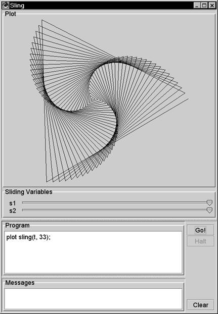 16.3.5 Adding Lines You can increase the number of lines in a plot by changing the value of the nLine variable. This variable establishes the number of lines in each plot. Figure 16.5 uses 2,000 lines to depict a rapidly spinning sling. Figure 16.5. Increasing a plot's precision. By setting a value for the nLine variable, you can increase the number of lines that the Sling IDE uses.  16.3.6 Cartesian Plots The Sling language is named for its most interesting function, but the language includes other functions that describe one- and two-dimensional functions of time, including cartesian . A Cartesian plot specifies separate functions for the x and y values of the path of a point. When you're working with one-dimensional functions, it is often useful to apply a scale() function. The value of a scale function varies linearly from its first parameter to its second parameter as time varies from to 1 . You can also say that a scale value varies between its parameters "during the course of a plot." For example, to specify that x should vary from -5 to 5 during the course of a plot, you can write x = scale(-5, 5); The Sling programming language includes the built-in value for pi , so you might also write x = scale(-pi, pi); You can create y as a function of x . Here's an example: y = sin(4*x); The variable y holds a sin function of 4*x . Its argument goes from -4*pi to 4*pi in the course of the plot, enough for four complete cycles of the sin function. You can tie the x and y functions together with a cartesian() function, which accepts two parameters: a source for x values and a source for y values. The complete program is x = scale(-pi, pi); y = sin(4*x); plot cartesian(x, y); Figure 16.6 shows the results of this program. Figure 16.6. A Cartesian plot. The cartesian function lets you define the x and y values of a point separately. Here, x goes from -pi to pi as Sling makes its plot, and y is a function of x .  16.3.7 Cartesians as Points Another use of the cartesian function is to model particular points, using a scale to draw a line between the points. For example, Figure 16.7 shows a net of straight lines. Figure 16.7. Using Cartesian functions as points. A cartesian function can contain a simple point, and a scale can create a line between a pair of such points.  16.3.8 Polar Plots The polar function in Sling is similar to the sling function, but the second argument is the angle of the sling rather than the number of rotations of the sling. Specifying the angle directly lets you make the angle of the plot constant. Consider plotting a line from the lower-left corner to the upper-right corner. The angle of this line is 45 degrees, or pi/2 radians. To appear as a line, you must let the strap out over time, so the Sling command is plot polar(t, pi/4); You can interpret this as, "Plot the path of a stone on a sling whose strap varies from to 1 during the course of the plot and that is at a constant angle of pi/2 ." The second argument to the polar function need not be a constant. An interesting effect is to let the sling strap oscillate. For example, to establish a function for an angle that makes one revolution, use the statement theta = 2*pi*t; Then you can make the length of the strap a constant plus a smaller length that oscillates: len = 1 + .5*sin(8*theta); During the course of a plot, the value 8*theta will vary from to 16*pi , which is equal to 8 rotations. The strap length will go in and out 8 times as the plot proceeds. If you rotate (or swing) the sling a number of times that is relatively prime to the number of times you let the strap in and out, you can produce a braiding effect. For example: plot polar(len, 3 * theta); plots a line that goes around the origin 3 times, crossing itself many times but rejoining itself only once. Figure 16.8 shows this effect, plotting the pattern twice for esthetic effect. Figure 16.8. A polar plot. The polar function takes two arguments: a radius (the length of a sling strap) and the arc of the stone. 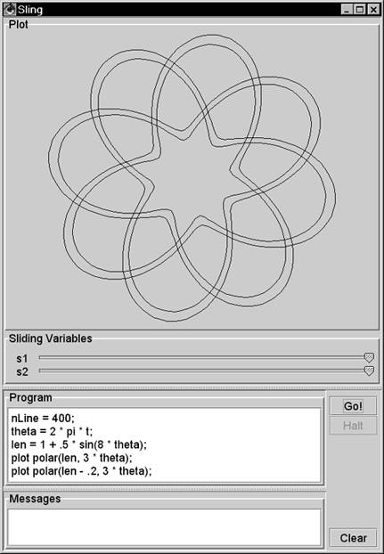 The difference between the sling function and the polar function is that the sling function assumes that you expect the strap to rotate. The sling function creates a result equivalent to taking a polar function and multiplying its angle argument by 2*pi*t . The program in Figure 16.8 is equivalent to the following version, which uses the sling function in lieu of the polar function: nLine = 400; theta = 2*pi*t; len = 1 + .5*sin(8*theta); plot sling(len, 3); plot sling(len - .2, 3); 16.3.9 For Loops For loops in Sling let you iterate a variable over a given range of integers. For example, Figure 16.9 uses a for loop to plot slings having different strap lengths. Figure 16.9. A for loop. The for loop shown executes its body for five different values of the variable r .  The parameters in a for command are a variable and two functions. The functions can be any sling functions, but integer values are most common. The Sling environment augments integers in a for loop to be two-dimensional functions of time. In Figure 16.9 the environment augments the "to" and "from" values to be cartesian(t, (0, 1)) and cartesian(t, (0, 5)) . The step of a for loop is always (1, 1) . Consider the program for (c, cartesian(3, 3), cartesian(7, 7)) { plot c + sling(1, 1); } This program steps the variable c through the values (3, 3) , (4, 4) , (5, 5) , (6, 6) and (7, 7) , drawing a sling around each of these centers. 16.3.10 Sliders The Sling development environment provides two sliders that let you experiment with many different variations of any program. For example, Figure 16.10 shows one of thousands of plots that result from the given program. Figure 16.10. Sling sliders. The Sling environment redisplays the plot almost continuously as the user moves the sliders. 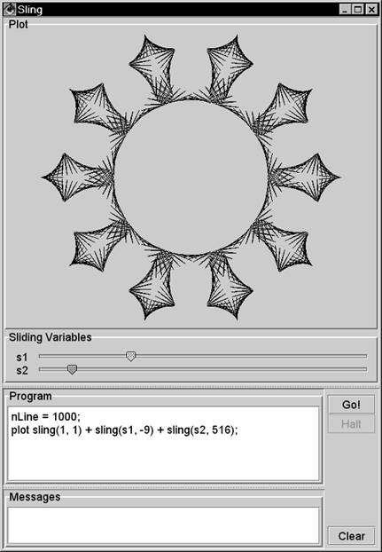 16.3.11 A Composite Example You can use the Sling IDE to explain to someone new to Sling the basic idea of how Sling works. In Figure 16.11, the slider s1 controls the degree of sweep around David's head. The slider s2 controls the size of the arc. Figure 16.11. An illustration of a sling. In this screen shot, the user has pulled the slider s1 nearly three-fourths of the way from right to left. The plot animates this movement, showing the stone's rotation as the user pulls the slider.  Here is the program for Figure 16.11: // crosshairs s = scale(-1.1, 1.1); plot cartesian(s, 0); plot cartesian(0, s); // arrow arc r = s2; angle = 2*pi * (1 - s1); plot polar(r, angle*t); // arrow head tip = polar(r, angle); plot tip + polar(.1*t, angle - pi/4); plot tip + polar(.1*t, angle - 3/4 * pi); // stone plot polar(1, angle) + sling(.1, 1); // sling strap plot polar(t, angle); The vertical and horizontal lines in the figure form crosshairs that identify the x and y axes. The variable s goes from -1.1 to 1.1 during the course of the plot. Two Cartesian plots lay out this line segment horizontally and vertically. The angle variable goes from to 2 * pi , as s1 goes fom 1 to . This arrangement gives the effect of the user pulling the sling around David's head. As the user pulls the slider from its initial, rightmost position, the stone circles around. The stone makes one full rotation if the user pulls the slider all the way to the left. The program describes the location of the tip of the arrow's head using polar(r, angle) . From this tip, the program plots two other polar functions that head off at an angle of pi/2 (90 degrees) from each other. The center of the stone is always 1 unit away from the center of the plot at polar(1, angle) . To this center, you attach a small sling function whose job is to draw the stone (the circle) in the plot. Each time the user moves the slider, you draw the whole stone, centered on the end of the strap. For the strap, you need a straight line at the calculated angle . To effect this, imagine a ray that goes from 0 to 1 with time, heading in the angle direction. A function for this ray is polar(t, angle) . If the first argument were a constant, the polar function would specify only one point and not a line to represent the strap. This program uses a variety of techniques to compose an interactive program that illustrates the path of a sling. 16.3.12 More Plots The idea of Sling is to have fun experimenting with your own programs and especially to play with the effects of the sliders. You can use the examples in this section to get started writing your own programs. In addition, the directory "Sling Programs" on the CD contains a few more examples. 16.3.13 The Elements of Sling Figure 16.12 summarizes the elements of Sling. Figure 16.12. The elements of Sling. Each of these elements can appear in a plot command, and each element can serve as an argument to any other element. 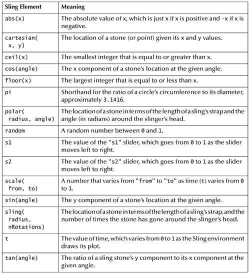 | 