2.3 A Simple Database Server Example

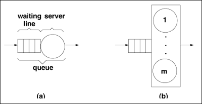
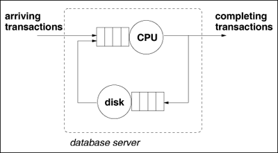
Consider a database server that has one CPU and one disk. Database transactions arrive to the database server for execution at a certain rate (e.g., 1.5 transactions per second (tps)). During its execution, a transaction alternates using the processor and the disk, quite likely more than once. At any point in time, one transaction might be using the CPU and another using the disk, while yet other transactions are waiting to use the CPU or disk. Thus, the CPU and the disk can each be characterized as a queue with a waiting line and a device that serves transactions. Figure 2.1 (a) shows a graphical representation used to illustrate a queue with a single resource server. Transactions arrive and wait if the resource is busy, otherwise they start using the resource immediately. In some cases, there is a single waiting line for multiple resources (e.g., a multiprocessor, a single line for multiple tellers at the bank). This type of queue is represented in Fig. 2.1 (b). Here, a transaction waits in line if all m resources are busy. As soon as a resource becomes available, it starts serving one of the transactions waiting in the queue.

Figure 2.1. (a) Single queue with one resource server (b) Single queue with m resource servers.

The notation just described can be used to represent a simple database server, as illustrated in Fig. 2.2. This figure depicts a network of queues, or Queuing Network (QN). Elements such as database transactions, HTTP requests, and batch jobs, that receive service from each queue in the QN are generically called customers. QNs are used throughout this book as a framework to think about performance at all stages within a system's life cycle.

Figure 2.2. Queuing network for a simple database server.

Mapping an existing system into a QN is not trivial. Models are usually built with a specific goal in mind. For instance, one may want to know how the response time of database transactions varies with the rate at which transactions are submitted to the database server. Or, one may want to know the response time if the server is upgraded. Good models abstract out some of the complexities of real systems while retaining what is essential to meet the model goals. For example, the QN model for the database server example abstracts the complexity of a rotating magnetic disk (e.g., disk controller, disk cache, rotating platter, arm) into a single resource characterized by a single parameter (i.e., the average number of I/Os that the disk can service per second). However, if one were interested in studying the effect of different disk architectures on performance, then the specific features of interest in the I/O architecture would have to be explicitly considered by the model.

In order to use a QN model of the database server to predict performance for a given transaction arrival rate (e.g., 1.5 tps) one needs to know how much time a typical transaction spends using the CPU and the disk (i.e., the total service time required by a transaction at the CPU and disk). The model is then used to compute the waiting time of a transaction at the CPU and at the disk. The total average service time of a transaction at a resource is called its service demand. This is an important notion that will be revisited many times in this book. Waiting times depend on service demands and on the system load (i.e., the average number of concurrent transactions in the system).