Section 9.2. Groups of Numbers
9.2. Groups of NumbersSpreadsheets are used to distil a few important pieces of information out of several pages of data. For example, say you want to hunt through a column looking for minimums and maximums, in order to find the lowest -priced product or best sales quarter. Or maybe you want to calculate averages, means, and percentile rankings to help grade a class of students. In either case, Excel provides a number of useful functions. Most of these are part of the Statistical group, although the SUM( ) function is actually part of the Math & Trig group . 9.2.1. SUM( ): Summing Up NumbersAlmost every Excel program in existence has been called on at least once to do the same thing: add a group of numbers. This task falls to the wildly popular SUM( ) function, which simply adds everything in it. The SUM( ) function takes over 200 arguments, each of which can be a single cell reference or a range of cells . Here's a SUM( ) formula that adds two cells: =SUM(A1,A2) And here's a SUM( ) formula that adds the range of 11 cells from A2 to A12: =SUM(A2:A12) And here's a SUM( ) formula that adds a range of cells along with a separately referenced cell, and two literal values: =SUM(A2:A12,B5,429.1,35000) Note: The SUM( ) function automatically ignores any cells in its range with text content, or any blank ones. However, SUM( ) adds up calendar dates (which are actually specially formatted numbers, as you saw in Section 2.2). Therefore, make sure you don't sum a range of cells that includes a date.
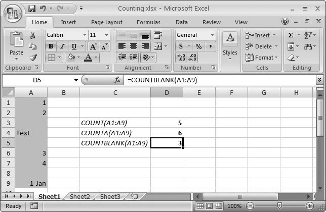
9.2.2. COUNT( ), COUNTA( ), and COUNTBLANK( ): Counting Items in a ListSometimes you don't need to add a series of cells, but instead want to know how many items there are (in a list, for instance). That's the purpose of Excel's straightforward counting functions, COUNT( ), COUNTA( ), and COUNTBLANK( ). COUNT( ) and COUNTA( ) operate similarly to the SUM( ) function in that they accept over 200 arguments, each of which can be a cell reference or a range of cells. The COUNT( ) function counts the number of cells that have numeric input (including dates). The COUNTA( ) function counts cells with any kind of content. And finally, the COUNTBLANK( ) function takes a single argumenta range of cellsand gives you the number of empty cells in that range (see Figure 9-3).
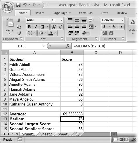
Here's how you could use the COUNT( ) function with a range of cells: =COUNT(A2:A12) For an example of when COUNT( ) comes in handy, consider the following formula, which determines the average of a group of cells, without requiring that you manually input the total number of values: =SUM(A2:A12)/COUNT(A2:A12) This formula finds the average of all the cells in the range A2:12 that have values. Because it uses COUNT( ), the average remains correct even if the range includes empty cells (which Excel simply ignores). Of course, Excel already includes an AVERAGE( ) function that can perform this calculation for you, but the COUNT( ) function is still useful in long lists of data that may contain missing information. For example, imagine you create a worksheet with a list of customer charges. One of the columns in your list is Discount Amount. Using the COUNT( ) function on the discount column, you can find out how many customers got a discount in your list. When you want to get a little fancier, use COUNT( ) on the Customer Name column to find out how many rows are in the table. Then you can divide the number of discount sales by the number of total sales to find out the percentage of the time that you sell something for a reduced price. You can also combine the counting functions to calculate some additional pieces of potentially useful information. If you subtract COUNT( ) from COUNTA( ), for example (that is, if your formula reads something like = COUNTA(A1:A10)COUNT(A1:A10) ), you end up with the number of text cells in the range. Tip: You can also use SUMIF( ) and COUNTIF( ) functions to sum or count cells that meet specific criteria. For more information on using conditional logic, as well as the SUMIF( ) and COUNTIF( ) functions, see pages 362 and 359, respectively. 9.2.3. MAX( ) and MIN( ): Finding Maximum and Minimum ValuesThe MAX( ) and MIN( ) functions pick the largest or smallest value out of a series of cells. This tool's great for picking important values (best-selling products, failing students, or historically high temperatures ) out of a long list of information. As with COUNT( ) and SUM( ), the MAX( ) and MIN( ) functions accept over 200 cell references or ranges. For example, the following formula examines four cells (A2, A3, B2, and B3) and tells you the largest value: =MAX(A2:B3) The MAX( ) and MIN( ) functions ignore any non-numeric content, which includes text, empty cells, and Boolean (true or false) values. Excel includes dates in MAX( ) and MIN( ) calculations because it stores them internally as the number of days that have passed since a particular date. (For Windows versions of Excel, this date is January 1, 1900; see Section 2.2 for details on how this works.) For this reason, it makes little sense to use MAX( ) or MIN( ) on a range that includes both dates and ordinary numeric data. On the other hand, you may want to use MAX( ) to find the most recent (that is, the largest) date or MIN( ) to find the oldest (or smallest) date. Just make sure you format the cell containing the formula using the Date number format (Section 5.1.2), so that Excel displays the date it has identified. Excel also provides MAXA( ) and MINA( ) functions, which work just like MAX( ) and MIN( ), except for the way in which they handle text and Booleans. MAXA( ) and MINA( ) always assume TRUE values equal 1 and FALSE values equal 0. Excel treats all text values as 0. For example, if you have a list of top professionals with a Salary column, and some cells say "Undisclosed," it makes sense to use MAX( ) and MIN( ) to ignore these cells altogether. On the other hand, if you have a list of items you've tried to auction off on eBay with a Sold For column, and some cells say "No Bids," you may use MINA( ) and MAXA( ) to treat this text as a 0 value. 9.2.4. LARGE( ), SMALL( ), and RANK( ): Ranking Your NumbersMAX( ) and MIN( ) let you grab the largest and smallest numbers, but what if you want to grab something in between? For example, you might want to create a top10 list of best-selling products, instead of picking out just the single best. In these cases, consider the LARGE( ) and SMALL( ) functions, which identify values that aren't quite the highest or lowest. In fact, these functions even let you specify how far from the top and bottom you want to look. Here's how they work. Both the LARGE( ) and SMALL( ) functions require two arguments: the range you want to search, and the item's position in the list. The list position is where the item would fall if the list were ordered from largest to smallest (for LARGE( )), or from smallest to largest (for SMALL( )). Here's what LARGE( ) looks like: LARGE(range, position) For example, if you specify a position of 1 with the LARGE( ) function, then you get the largest item on the list, which is the same result as using MAX( ). If you specify a position of 2, as in the following formula, then you get the second largest value: =LARGE(A2:A12, 2) Here's an example formula that adds the three largest entries in a range: =LARGE(A2:A12,1) + LARGE(A2:A12,2) + LARGE(A2:A12,3) Assuming the range A2:A12 contains a list of monthly expenses, this formula gives you the total of your three most extravagant splurges. SMALL( ) performs the opposite task by identifying the number that's the smallest, second-smallest, and so on. For example, the following formula gives you the second-smallest number: =SMALL(A2:A12, 2) And finally, Excel lets you approach this problem in reverse. Using the RANK( ) function, you can find where a specific value falls in the list. The RANK( ) function requires two parts : the number you're looking for and the range you're searching. In addition, you can supply a third parameter that specifies how Excel should order the values before searching. (By default, Excel searches values from highest to lowest.) Here's what the RANK( ) formula looks like: RANK(number, range, [order_type]) For example, imagine you have a range of cells from A2 to A12 that represent scores on a test. Somewhere in this range is a score of 77. You want to know how this compares to the other marks, so you create the following formula using the RANK( ) function: =RANK(77, A2:A12) If this formula works out to 5, you know that 77 is the fifth-highest score in the range you indicated. But what if more than one student scored 77? Excel handles duplicates in much the same way as it deals with tied times in races. If three students score 77, for example, then they all tie for fifth place. But the next lowest grade (say, 75) gets a rank of eightthree positions down the list. If you want to rank values in the reverse order, then you need to include a third argument of 0. This orders them from lowest to highest (so that rank 1 has the lowest grade): =RANK(77, A2:A12, 0) Note: If you use RANK( ) to rank a number that doesn't exist in the data series, Excel gives you the #N/A error code in the cell, telling you it can't rank the number because the number isn't there. You can do a neat trick and rank all your numbers in a list. For example, assume you have a list of grades in cells A2 to A12. You want to show the rank of each grade in the corresponding cells B2 to B12. Calculate the rank for A2 like so: =RANK(A2, $A:$A) This formula uses absolute references for the list. That means you can copy this formula to cells B3 through B12 to calculate the rank for the remaining grades, and Excel automatically adjusts the formula to what you need. 9.2.5. AVERAGE( ) and MEDIAN( ): Finding Average or Median ValuesExcel makes it easy for you to find the average value for a set of numbers. The AVERAGE( ) function doesn't accomplish anything you couldn't do on your own using COUNT( ) and SUM( ) together, but, well, you could also bake your own bread. Bottom line: the AVERAGE( ) function is a real timesaver. The AVERAGE( ) function uses just one argument: the cell range you want to average: =AVERAGE(A2:A12) The AVERAGE( ) function ignores all empty cells or text values. For example, if the preceding formula had only three numbers in the range A2:A12, then Excel would add these values and divide them by 3. If this isn't the behavior you want, you can use the AVERAGEA( ) function, which counts all text cells as though they contain the number 0 (but it still ignores blank cells). (For an example of when text should and shouldn't be treated as 0 values, see Section 9.2.3.) Tip: In some cases, you may want to perform an average that ignores certain values. For example, when determining the average score of all students on a test, you may want to disregard students who scored 0 because they may have been absent. In this case, you can use the conditional averaging technique described in Section 13.1.3. Excel can also help you identify the median value for a set of numbers. If you were to order your range of numbers from lowest to highest, then the median would be the number that falls in the middle. (If you have an even amount of numbers, Excel averages the two middle numbers to generate the median.) You calculate the median (see Figure 9-4) in the same way that you calculate an average: =MEDIAN(A2:A12)
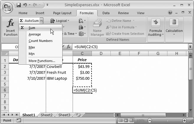
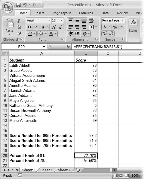
Tip: Remember, Excel offers a quick shortcut for five of its most popular functionsSUM( ), AVERAGE( ), COUNT( ), MAX( ), and MIN( ). Just choose Formulas  Function Library AutoSum to perform a quick sum on any group of selected cells. Or, if you click the drop-down arrow on this button, you see a list where you can quickly unleash any of the other four functions. Function Library AutoSum to perform a quick sum on any group of selected cells. Or, if you click the drop-down arrow on this button, you see a list where you can quickly unleash any of the other four functions. 9.2.6. MODE( ): Finding Numbers That Frequently Occur in a List MODE( ) is an interesting function that gives you the most frequently occurring value in a data series. For example, if you use MODE( ) with the worksheet shown in Figure 9-4 like this: = MODE(B2:B10) , you get the number 78. That's because the score 78 occurs twice, unlike all the other scores, which just appear once. MODE( ) does have a few limitations, though. It ignores text values and empty cells, so you can't use it to get the most common text entry. It also returns the error code #N/A if no value repeats at least twice. And if there's more than one value that repeats the same number of times, then you get the highest number. 9.2.7. PERCENTILE( ) and PERCENTRANK( ): Advanced Ranking FunctionsIf you really want to dissect the test scores from the worksheet in Figure 9-4, you don't need to stop with simple averages, medians, and rankings. You can take a closer look at the overall grade distribution by using the PERCENTILE( ) and PERCENTRANK( ) functions. People often use percentiles to split groups of students into categories. (Technically, a percentile is a value on a scale of 1 to 100, indicating the percentage of scorers in any given ranking who are equal to, or below, the scorer in question.) For example, you might decide that the top 10 percent of all the students in your class will gain admission into an advanced class the following semester. In other words, a student's final grade must be better than 90 percent of his or her classmates. Students at this prestigious level occupy the 90th percentile. That's where the PERCENTILE( ) function comes in very handy. You supply the cell range, the percentile (as a fraction from 0 to 1), and the function reveals the numeric grade the student needs to match that percentile. For example, here's how you'd calculate the minimum grade needed to enter the 90th percentile (assuming the grades are in cells B2 to B10): =PERCENTILE(B2:B10, 0.9) Percentiles make the most sense when you have a large number of values because then the distribution becomes the most regular. In other words, there's a wide range of different test scores that are well spread out, with no " clumping " that may skew your results. Percentiles don't work as well with small amounts of data. For example, if you have fewer than 10 students and try to calculate the grade needed to enter the 90th percentile, then you'll come up with a grade higher than any student has scored so far (and possibly higher than 100 percent). PERCENTRANK( ) performs the inverse task. It takes a range of data and a number from 1 to 100, and gives you the fraction indicating the number's percentile. The following formula, for instance, returns the percentile of the grade 81 (as it compares to a list of other grades): =PERCENTRANK(B2:B13,81) Using the data shown in Figure 9-5, this formula gives you the fraction 0.727, indicating that an 81 falls into the 72nd percentile (and almost hits the 73rd percentile). That is, it's a better score than 72 percent of all the other students, and a lower score than the other 28 percent. In this case, you can also apply the rounding functions explained earlier in the chapter because percentiles are (by convention) whole numbers. You can use ROUND( ) to round the result of the formula to the closest percentile (73rd), or use TRUNC( ) to return the highest percentile that the student actually reached (72nd), which is the conventional approach.
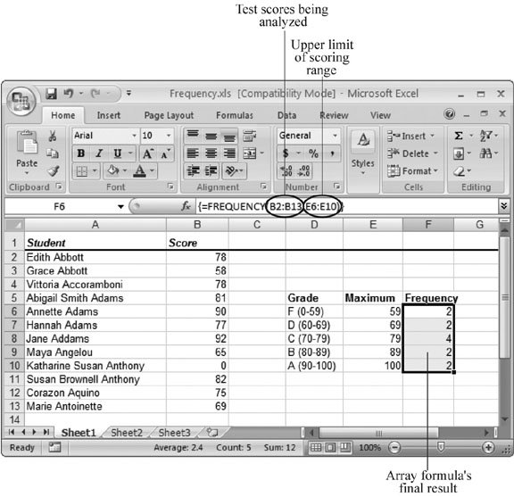
9.2.8. FREQUENCY( ): Identifying to Which Category a Number BelongsThe FREQUENCY( ) function is the last statistical function you'll learn about in this section. Like the functions you've seen so far, FREQUENCY( ) helps you analyze numbers based on the way they're distributed within a group of other numbers. For example, PERCENTILE( ) and PERCENTRANK( ) let you examine how a single test score ranks in comparison to other students' scores. Functions like AVERAGE(), RANK( ), and MEDIAN( ) give you other tools to compare how different values stack up against one another. FREQUENCY( ) is different from these functions in one key way: It doesn't compare values against each other. Instead, it lets you define multiple ranges, and then, after chewing through a list of numbers, tells you how many values on the list fall into each range. For example, you could use FREQUENCY( ) to examine a list of incomes in order to see how many belong in a collection of income ranges that you've identified. FREQUENCY( ) is a little more complicated than the other functions you've seen in this chapter because it gives you what's known as an array (a list of separate values). When a function gives you an array, it returns multiple results that must be displayed in different cells. In order to use the FREQUENCY( ) function properly, you first need to create an array formula , which displays its results in a group of cells. (Put another way: A plain- vanilla formula occupies one cell; an array formula spans multiple cells.) A worksheet filled with student test scores, such as the one shown in Figure 9-6, provides an ideal place to learn how the FREQUENCY( ) function works, showing you how many students aced a test and how many botched it. Here's how to use the FREQUENCY( ) function to generate the results shown in cells F6 through F10:
|