Section 8.1. Creating a Basic Formula
8.1. Creating a Basic FormulaFirst things first: what exactly do formulas do in Excel? A formula is a series of mathematical instructions that you place in a cell in order to perform some kind of calculation. These instructions may be as simple as telling Excel to sum up a column of numbers , or they may incorporate advanced statistical functions to spot trends and make predictions . But in all cases, all formulas share the same basic characteristics:
One of the simplest formulas you can create is this one: =1+1 The equal sign's how you tell Excel that you're entering a formula (as opposed to a string of text or numbers). The formula that follows is what you want Excel to calculate. Note that the formula doesn't include the result . When creating a formula in Excel, you write the question, and then Excel coughs up the answer, as shown in Figure 8-1.
All formulas use some combination of the following ingredients :
Table 8-1. Excel's Arithmetic Operators
Note: The percentage (%) operator divides a number by 100. 8.1.1. Excel's Order of OperationsFor computer programs and human beings alike, one of the basic challenges when it comes to reading and calculating formula results is figuring out the order of operations mathematician -speak for deciding which calculations to perform first when there's more than one calculation in a formula. For example, given the formula: =10 - 8 * 7 the result, depending on your order of operations, is either 14 or46. Fortunately, Excel abides by what's come to be accepted among mathematicians as the standard rules for order of operations, meaning it doesn't necessarily process your formulas from left to right. Instead, it evaluates complex formulas piece-by-piece in this order:
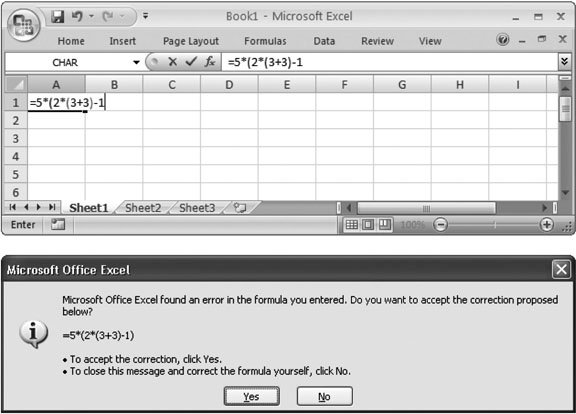
Note: When Excel encounters formulas that contain operators of equal precedence (that is, the same order of operation priority level), it evaluates these operators from left to right. However, in basic mathematical formulas, this has no effect on the result. For example, consider the following formula: =5 + 2 * 2 ^ 3 - 1 To arrive at the answer of 20, Excel first performs the exponentiation (2 to the power of 3): =5 + 2 * 8 - 1 and then the multiplication: =5 + 16 - 1 and then the addition and subtraction: =20 To control this order, you can add parentheses. For example, notice how adding parentheses affects the result in the following formulas: 5 + 2 * 2 ^ (3 - 1) = 13 (5 + 2) * 2 ^ 3 - 1 = 55 (5 + 2) * 2 ^ (3 - 1) = 28 5 + (2 * (2 ^ 3)) - 1 = 20 You must always use parentheses in pairs (one open parenthesis for every closing parenthesis). If you don't, then Excel gets confused and lets you know you need to fix things, as shown in Figure 8-2. Tip: Remember, when you're working with a lengthy formula, you can expand the formula bar to see several lines at a time. To do so, click the down arrow at the far right of the formula bar (to make it three lines tall), or drag the bottom edge of the formula bar to make it as many lines large as you'd like. Section 1.3.3 shows an example.
8.1.2. Cell ReferencesExcel's formulas are handy when you want to perform a quick calculation. But if you want to take full advantage of Excel's power, then you're going to want to use formulas to perform calculations on the information that's already in your worksheet. To do that you need to use cell references Excel's way of pointing to one or more cells in a worksheet. For example, say you want to calculate the cost of your Amazonian adventure holiday, based on information like the number of days your trip will last, the price of food and lodging, and the cost of vaccination shots at a travel clinic. If you use cell references, then you can enter all this information into different cells, and then write a formula that calculates a grand total. This approach buys you unlimited flexibility because you can change the cell data whenever you want (for example, turning your three-day getaway into a month-long odyssey ), and Excel automatically refreshes the formula results. Cell references are a great way to save a ton of time. They come in handy when you want to create a formula that involves a bunch of widely scattered cells whose values frequently change. For example, rather than manually adding up a bunch of subtotals to create a grand total, you can create a grand total formula that uses cell references to point to a handful of subtotal cells. They also let you refer to large groups of cells by specifying a range . For example, using the cell reference lingo you'll learn in Section 8.1.4.3, you can specify all the cells in the first column between the 2nd and 100th rows. Every cell reference points to another cell. For example, if you want a reference that points to cell A1 (the cell in column A, row 1), then use this cell reference: =A1 In Excel-speak, this reference translates to "get the value from cell A1, and insert it in the current cell." So if you put this formula in cell B1, then it displays whatever value's currently in cell A1. In other words, these two cells are now linked. Cell references work within formulas just as regular numbers do. For example, the following formula calculates the sum of two cells, A1 and A2: =A1+A2 Note: In Excel lingo, A1 and A2 are precedents , which means another cell needs them to perform a calculation. Cell B1, which contains the formula, is called the dependent , because it depends on A1 and A2 to do its work. These terms become important when you need to hunt for errors in a complex calculation using Excel's error-checking tools (Section 13.5). Provided both cells contain numbers, you'll see the total appear in the cell that contains the formula. If one of the cells doesn't contain numeric information, then you'll see a special error code instead that starts with a # symbol. Errors are described in more detail in Section 8.1.5. Note: This chapter focuses on how to perform calculations using cells that contain ordinary numbers. Excel also lets you manipulate other types of content in a formula, like text and dates. You'll learn more about these topics in Chapter 11.
8.1.3. How Excel Formats Cells That Contain Cell ReferencesAs you learned in Chapter 5, the way you format a cell affects how Excel displays the cell's value. When you create a formula that references other cells, Excel attempts to simplify your life by applying automatic formatting. It reads the number format that the source cells (that is, the cells being referred to ) use, and applies that to the cell with the formula. If you add two numbers and you've formatted both with the Currency number format, then your result also has the Currency number format. Of course, you're always free to change the formatting of the cell after you've entered the formula. Usually, Excel's automatic formatting is quite handy. Like all automatic features, however, it's a little annoying if you don't understand how it works when it springs into action. Here are a few points to consider:
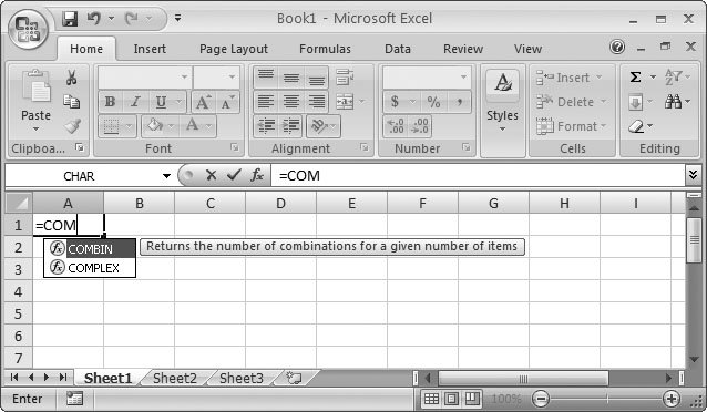
8.1.4. FunctionsA good deal of Excel's popularity is due to the collection of functions it provides. Functions are built-in, specialized algorithms that you can incorporate into your own formulas to perform powerful calculations. Functions work like miniature computer programsyou supply the data, and the function performs a calculation and gives you the result. In some cases, functions just simplify calculations that you could probably perform on your own. For example, most people know how to calculate the average of several values, but when you're feeling a bit lazy, Excel's built-in AVERAGE( ) function automatically gives you the average of any cell range. Even more usefully, Excel functions perform feats that you probably wouldn't have a hope of coding on your own, including complex mathematical and statistical calculations that predict trends hidden relationships in your data that you can use to make guesses or predict the future. Tip: You can create your own Excel functions by writing a series of instructions using VBA (Visual Basic for Applications) code. Chapter 28 shows you how. Every function provides a slightly different service. For example, one of Excel's statistical functions is named COMBIN( ). It's a specialized tool used by probability mathematicians to calculate the number of ways a set of items can be combined. Although this sounds technical, even ordinary folks can use COMBIN( ) to get some interesting information. You can use the COMBIN( ) function, for example, to count the number of possible combinations there are in certain games of chance. The following formula uses COMBIN( ) to calculate how many different five-card combinations there are in a standard deck of playing cards: =COMBIN(52,5) Functions are always written in all-capitals. (More in a moment on what those numbers inside the parentheses are doing.) However, you don't need to worry about the capitalization of function names because Excel automatically capitalizes the function names that you type in (provided it recognizes them).
8.1.4.1. Using a function in a formulaFunctions alone don't actually do anything in Excel. Functions need to be part of a formula to produce a result. For example, COMBIN( ) is a function name. But it actually does somethingthat is, give you a resultonly when you've inserted it into a formula, like so: =COMBIN(52,5) . Whether you're using the simplest or the most complicated function, the syntax or, rules for including a function within a formulais always similar. To use a function, start by entering the function name. Excel helps you out by showing a pop-up list with possible candidates as you type, as shown in Figure 8-3. This handy feature, Formula AutoComplete, is new to Excel 2007.
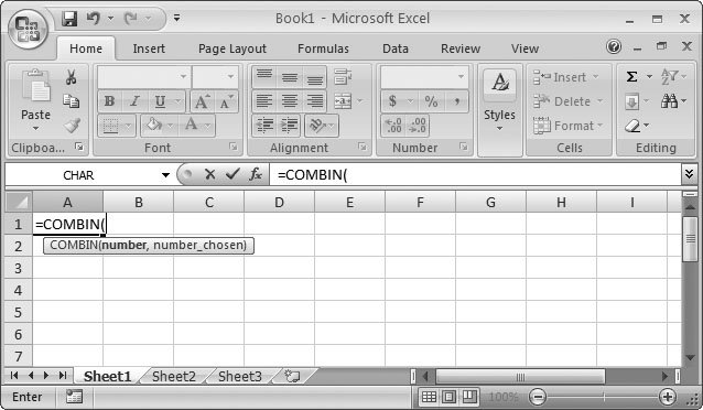
After you type the function name, add a pair of parentheses. Then, inside the parentheses, put all the information the function needs to perform its calculations. In the case of the COMBIN( ) function, Excel needs two pieces of information, or arguments . The first is the number of items in the set (the 52-card deck), and the second's the number of items you're randomly selecting (in this case, 5). Most functions, like COMBIN( ), require two or three arguments. However, some functions can accept many more, while a few don't need any arguments at all. Once again, Formula AutoComplete guides you by telling you what arguments you need, as shown in Figure 8-4. Once you've typed this formula into a cell, the result (2598960) appears in your worksheet. In other words, there are 2,598,960 different possible five-card combinations in any deck of cards. Rather than having to calculate this fact using probability theoryor, heaven forbid , trying to count out the possibilities manuallythe COMBIN( ) function handled it for you.
Note: Even if a function doesn't take any arguments, you still need to supply an empty set of parentheses after the function name. One example is the RAND( ) function, which generates a random fractional number. The formula =RAND( ) works fine, but if you forget the parentheses and merely enter =RAND , then Excel displays an error message ( #NAME ?) that's Excelian for: "Hey! You got the function's name wrong." See Table 8-2 for more information about Excel's error messages.
8.1.4.2. Using cell references with a functionOne of the particularly powerful things about functions is that they don't necessarily need to use literal values in their arguments. They can also use cell references. For example, you could rewrite the five-card combination formula (mentioned above) so that it specifies the number of cards that'll be drawn from the deck based on a number that you've typed in somewhere else in the spreadsheet. Assuming this information's entered into cell B2, the formula would become: =COMBIN(52, B2 ) Building on this formula, you can calculate the probability (albeit astronomically low) of getting the exact hand you want in one draw: =1/COMBIN(52,B2) You could even multiply this number by 100 or use the Percent number style to see your percentage chance of getting the cards you want. Tip: Excel gives you a detailed function reference to find functions and learn about them. Excel's information doesn't make for light reading, though; for the most part, it's in IRS-speak. You'll learn more about using this reference in Section 8.2.4. 8.1.4.3. Using cell ranges with a functionIn many cases, you don't want to refer to just a single cell, but rather a range of cells. A range is simply a grouping of multiple cells. These cells may be next to each other (say, a range that includes all the cells in a single column), or they could be scattered across your worksheet. Ranges are useful for computing averages, totals, and many other calculations. To group together a series of cells, use one of the three following reference operators:
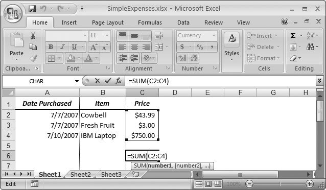
Tip: As you might expect, Excel lets you specify ranges by selecting cells with your mouse, instead of typing in the range manually. You'll see this trick later in this chapter in Section 5.1.4.4. You can't enter ranges directly into formulas that just use the simple operators. For example, the formula = A1:B1+5 doesn't work, because Excel doesn't know what to do with the range A1:B1. (Should the range be summed up? Averaged? Excel has no way of knowing.) Instead, you need to use ranges with functions that know how to use them. For instance, one of Excel's most basic functions is named SUM( ); it calculates the total for a group of cells. To use the SUM( ) function, you enter its name, an open parenthesis, the cell range you want to add up, and then a closed parenthesis. Here's how you can use the SUM( ) function to add together three cells, A1, A2, and A3: =SUM(A1,A2,A3) And here's a more compact syntax that performs the same calculation using the range operator: =SUM(A1:A3) A similar SUM( ) calculation's shown in Figure 8-5. Clearly, if you want to total a column with hundreds of values, it's far easier to specify the first and last cell using the range operator rather than including each cell reference in your formula!
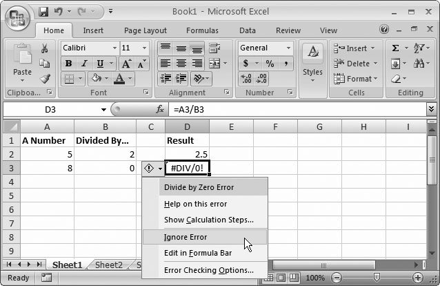
Sometimes your worksheet may have a list with unlimited growth potential, like a list of expenses or a catalog of products. In this case, you can code your formulas to include an entire column by leaving out the row number. For example, the range A:A includes all the cells in column A (and, similarly, the range 2:2 includes all the cells in row 2). The range A:A also includes any heading cells, which isn't a problem for the SUM( ) function (because it ignores text cells), but could cause problems for other functions. If you don't want to include the top cell, then you need to think carefully about what you want to do. You could create a normal range that stretches from the second cell to the last cell using the mind-blowingly big range A2:A1048576. However, this could cause a problem with older versions of Excel, which don't support as many rows. You're better off creating a table (described in Chapter 14). Tables expand automatically, updating any linked formulas. 8.1.5. Formula ErrorsIf you make a syntax mistake when entering a formula (such as leaving out a function argument or including a mismatched number of parentheses), Excel lets you know right away. Moreover, like a stubborn school teacher, Excel won't accept the formula until you've corrected it. It's also possible, though, to write a perfectly legitimate formula that doesn't return a valid answer. Here's an example: =A1/A2 If both A1 and A2 have numbers, this formula works without a hitch. However, if you leave A2 blank, or if you enter text instead of numbers, then Excel can't evaluate the formula, and it reminds you with an error message. Excel lets you know about formula errors by using an error code that begins with the number sign (#) and ends with an exclamation point (!), as shown in Figure 8-6. In order to remove this error, you need to track down the problem and resolve it, which may mean correcting the formula or changing the cells it references.
When you click the exclamation mark icon next to an error, you see a menu of choices (as shown in Figure 8-6):
Note: Sometimes a problem isn't an error, but simply the result of data that hasn't yet been entered. In this case, you can solve the problem by using a conditional error-trapping formula . This conditional formula checks if the data's present, and it performs the calculation only if it is. The next section, "Logical Operators," shows one way to use an error-trapping formula. Table 8-2 lists the error codes that Excel uses. Table 8-2. Excel's Error Codes
Note: Chapter 13 describes a collection of Excel tools designed to help you track down the source of an error in a complex formulaespecially one where the problem isn't immediately obvious. 8.1.6. Logical OperatorsSo far, you've seen the basic arithmetic operators (which are used for addition, subtraction, division, and so on) and the cell reference operators (used to specify one or more cells). There's one final category of operators that's useful when creating formulas: logical operators . Logical operators let you build conditions into your formulas so the formulas produce different values depending on the value of the data they encounter. You can use a condition with cell references or literal values. For example, the condition A2=A4 is true if cell A2 contains the same value as cell A4. On the other hand, if these cells contain different values (say 2 and 3), then the formula generates a false value. Using conditions is a stepping stone to using conditional logic. Conditional logic lets you perform different calculations based on different scenarios. For example, you can use conditional logic to see how large an order is, and provide a discount if the total order cost's over $5,000. Excel evaluates the condition, meaning it determines if the condition's true or false. You can then tell Excel what to do based on that evaluation. Table 8-3 lists all the logical operators you can use to build formulas. Table 8-3. Logical Operators
You can use logical operators to build standalone formulas, but that's not particularly useful. For example, here's a formula that tests whether cell A1 contains the number 3: =(A2=3) The parentheses aren't actually required, but they make the formula a little bit clearer, emphasizing the fact that Excel evaluates the condition first, and then displays the result in the cell. If you type this formula into the cell, then you see either the uppercase word TRUE or FALSE, depending on the content in cell A2. On their own, logical operators don't accomplish much. However, they really shine when you start combining them with other functions to build conditional logic. For example, you can use the SUMIF( ) function, which totals the value of certain rows, depending on whether the row matches a set condition. Or you can use the IF( ) function to determine what calculation you should perform. The IF( ) function has the following function description: IF(condition, [value_if_true], [value_if_false]) In English, this line of code translates to: If the condition is true, display the second argument in the cell; if the condition is false, display the third argument. Consider this formula: =IF(A1=B2, "These numbers are equal", "These numbers are not equal") This formula tests if the value in cell A1 equals the value in cell B2. If this is true, you'll see the message "These numbers are equal" displayed in the cell. Otherwise, you'll see "These numbers are not equal". Note: If you see a quotation mark in a formula, it's because that formula uses text. You must surround all literal text values with quotation marks. (Numbers are different: You can enter them directly into a formula.) People often use the IF( ) function to prevent Excel from performing a calculation if some of the data is missing. Consider the following formula: =A1/A2 This formula causes a divide-by-zero error if A2 contains a 0 value. Excel then displays an error code in the cell. To prevent this from occurring, you can replace this formula with the conditional formula shown here: =IF(A2=0, 0, A1/A2) This formula checks if cell A2 is empty or contains a 0. If so, the condition's true, and the formula simply gives you a 0. If it isn't, then the condition's false, and Excel performs the calculation A1/A2. Practical examples of conditional logic abound in Chapters 12 and 13.
|

 Clipboard