Simulation

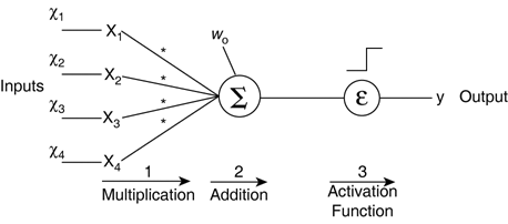
Perceptrons are in fact function approximators, denoted y = f(x). The process of simulation or computing the function f involves filtering an input pattern x through the network to get the corresponding output y. This is done in two stages: computing the net sum and applying the activation function.

The Net Sum

The first part involves determining the net sum, denoted with the Greek zeta z. This is the addition (denoted by the Greek sigma S) of all the inputs multiplied by their weights (x_iw_i):

The first statement equivalent to z assumes the first input is grounded at x₀ = 1 to represent the bias. The second statement shows the offset w₀ explicitly (see Figure 17.3). This is to remind ourselves that it's there and should not be forgotten!

Figure 17.3. Outline of the operations used for computing the output of a perceptron, based on the input pattern.

Generally speaking, the process that combines all the weighted inputs is called a combination function. In theory, this can be almost any function, but in practice, a sum is used most often. This has many advantages for the learning by keeping the model simple.

Activation

After the net sum z has been computed, it can be used to determine the output y. The only thing left to do is to pass the result through an activation function, usually noted s (lowercase Greek sigma):

In the original perceptron, this activation function outputs a result based on the sign of the net sum z. If it is positive, the output is set to 1, and 0 corresponds to a negative net sum:

Generally, it's beneficial to keep the result as a continuous value rather than restrict it to two discrete values. This mainly allows continuous numbers to be used in the problem at hand (for instance, smooth movement control), but can also be easier to deal with during training. It's also feasible to have both; a binary output is computed, and training is based on the net sum z. Early variations of the Adaline did this.

Further Information

Many other smooth functions are used for activation. These are generally nonlinear functions corresponding to a smooth curve within [0,1]. Such functions have little benefit for single-layer perceptrons, but prove essential when multiple perceptrons are cascaded. Chapter 19, "Multilayer Perceptrons," discusses these in depth.

Algorithm Outline

Listing 17.1 shows an outline of the algorithm in pseudo-code almost as long as the actual implementation! It assumes that there are two initialized arrays (input and weight) and an activation function.

Listing 17.1 Computing the Output of a Single Perceptron

 net_sum = 0 for all i      net_sum += input[i] * weight[i] end for output = activation( net_sum ) 

The output is often used as the prediction of an arbitrary function of the inputs. For example, the output may evaluate the suitability of a behavior or determine whether a situation is dangerous. We'll discuss in much more detail how to use this result, and show how to it can be applied in practice later. For the moment, we need to know how to train the perceptron to approximate a function correctly regardless of its use. This is done by optimizing each of the weights in the network.