The Great Divide

---

Capacity Planning

In a previous chapter we discussed how to plan for your initial backup architecture, including the following considerations:

• What data to back up

• How much data to back up

• The rate of change for that data

Capacity planning is a very similar but easier exercise, since we have most of the information already in our hands. Using the information gathered during your interview of the data owners, you should be able to extrapolate an estimation of how fast the data will grow. Most database administrators that we have talked to have a very good idea of the percentage of growth within their databases. Make sure you ask these questions during your initial interview phase with them to make this part of your capacity planning go as smooth as possible. Here are a few sample questions to ask data owners:

• How large is your data/database?

• What percentage of change happens to your data daily?

• Is there a particular point when the data changes more than usual?

• How much of that change is actual data growth?

• Can you anticipate an annual percentage of growth?

• What are your recovery expectations?

The most important part of capacity planning is determining where your data plateaus during the backup schedules and retentions you have subscribed. It is the plateau that will allow you to properly size your environment. The charts and tables to follow graphically represent the equations we have used to arrive at the results found in our examples. Even though these equations look daunting, trust us, it is only math and we will explain in detail how we are achieving these numbers.

Table 9.1 shows a sample of some of the data we have collected at a client site with regard to growth and capacity planning. To make things easy, we converted frequency and retention levels to days.

Table 9.1: Capacity Planning Chart

SERVER	AMOUNT OF DATA	FULL FREQUENCY (DAYS)	RETENTION (DAYS)
Mammoth	~100 GB	7	28

INCREMENTAL FREQUENCY (DAYS)	RETENTION (DAYS)	PERCENTAGE OF CHANGE	REQUIRED STORAGE
1	14	10%	520 GB

Here we will present to you the formulae used to calculate the required backup storage media need for the server, Mammoth, based on the maximum retention level, or 28 days. The percentage of change comes from our initial interview of the data owners, who may know the estimated percentage of change, or by simply taking a rough estimate, for the sake of example we are going to use 10 percent as our rate of change. While this rate of change may seem high or low, it makes the examples much easier to visualize. If you are using VERITAS NetBackup, you may use their File System Analyzer tool, which may give you a more accurate view.

The chart in Figure 9.1 visually represents the equation used to define the total capacity required for the full backups. While you may not need a chart to understand how much data a full backup will take, this graphic and these equations are a consistent method for which to use in modeling your backups.

Let's take some time to understand the Backup Models. The top portion of the figure is a graph that represents the days along the x-axis (1-33), with the data (D-Amount of data backed up) backed up running along the pos-y-axis and the data changed (pD) along the neg-y-axis. Whenever we use an arrow in the positive direction on the y-axis, it represents a backup that has been run, while an arrow in the negative direction on the y-axis represents changed data (pD, where p is the rate of change and D is the amount of data). Notice the Ff (Full-frequency) between #1 and #2, this represents the number of days between scheduled full backup jobs. Also note none of the changed data (pD) is being backed up. Since this is a Full Backup Model no distinction is made between changed data and unchanged data as with the Incremental Models discussed later.

The Total Backup graph shown directly below it presents a graphical view of how we reach our data plateaus and when. As you can see from the chart, Full Backups performed every 7 days and retained for 28 days means that we will need 4D or 4 times the total amount of data backed up with each Full. A much easier way to look at this is the formula. If we keep the fulls for twenty-eight days, then we will have a maximum of four full backups stacked at any one time. Using our example, 4D or 400GB will be required for this one client based on the policy requirements subscribed to. The incremental backups become a bit more interesting as you will see in the following charts and graphs.

Now again in Figure 9.2, we have the familiar 33-day graph, with Data (D) backed up traveling on the positive y-axis and the changed data (pD) traveling on the negative y-axis. Notice once again, Ff is the number of days between scheduled full backup jobs and now we have introduced If or the number of days between scheduled incremental backup jobs. This time we do show changed data (pD) being backed up because this is a Differential Incremental Backup Model.

For the next example we retain the differential incremental backups for 14 days. These numbers are typical of most customer sites we have visited, so it's interesting to view these backup models because it paints a very clear picture of how much tape you actually require for your backup jobs. Day one we have a full, so the bottom graph does not show an incremental backup; however, on day two we backup pD, which again is the rate of change × Total Data being backed up. This continues for as long as the Incremental frequency defines itself or until a Full backup is required to run, which you can see happens on day 8 of the bottom graph shown by a dotted line box. Notice our plateau is roughly 3× the amount of data we are backing up.

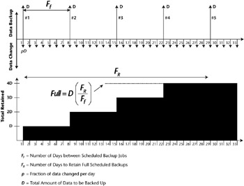
Figure 9.1: Full Backup Model.

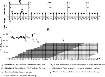
Figure 9.2: Differential Incremental Backup Model.

Finally a cumulative incremental will backup data changed since the last full backup. In our example here we are retaining our cumulative incremental backups for only seven days, not the 14 days as previously used by the differential example. The reason we decided on 7 is due to the sheer volume of data a cumulative would retain. You will quickly appreciate our decision as you look at the graph. Remember, the key here is where does our data plateau. Day one, as shown in the top graph, is our full backup, day 2 is pD or rate of change*Data, day 3 is 2pD, day 4, 3pD and so on. Since a cumulative incremental adds data changed from the last full, the amount of data required becomes significant. Essentially we are looking for the total data required for a cumulative incremental to be (p*D)+(2p*D)+ (3p*D)+(4p*D)+(5p*D)+(6p*D). So you can see from our bottom graph that by the seventh day we are past 2x the total Data being backed up by the full, unlike the Differential Incremental where it took us approximately two weeks to reach that point. With that being said, it may be prudent to perform full backup jobs more often if cumulative incremental is your preferred method, this should greatly reduce the amount of tapes required for your backups. Now if you retain your cumulative backups for 14 days, you simply would IR/Ff*Cinc (cumulative incremental).

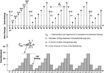
Figure 9.3: Cumulative Incremental Backup Model.

As a matter of practice we have included a proof for the differential incremental equation in Figure 9.4.

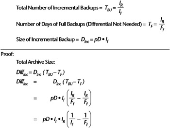
Figure 9.4: Proof of Differential Archive Size.

Grab a piece of paper and your number 2 pencil and follow along with the proof. Math is a wonderful thing.

So as you can see, capacity planning is made much easier by employing these charts, graphs, and equations. After you set up your favorite spreadsheet application with these formulae you can begin to model your environment based on estimated growth and proactively plan accordingly. Incidentally, since other backup tools allow you to do similar types of backups, you should be able to use these formulae to apply to those environments as well.

Note 

As a reminder, a cumulative incremental backs up all changed files since the last full backup. Differential incremental backs up all changed files since the last backup.

Note 

Using the information gathered during the interview process of the data owners should allow you to extrapolate an estimation of how fast the data will grow.

Using the plateaus as your guide, this client will require approximately 520 GB of storage to sustain the full and differential incremental retentions subscribed to in the policy and 610 GB for the full plus a cumulative incremental. Now if you have schedules that run once a month or once a year, these calculations should work as well, but the real girth of your required storage will be in your weekly full and daily incremental backups. If you are using a solution that employs the incremental-forever paradigm, you should still be able to apply these formulae to help you size your environment.

By taking all of the numbers for all of your clients, which you so masterfully calculated using your favorite spreadsheet, and multiplying them by the percentage of growth that you were able to ascertain from the data owners, you can plan for expansion by extrapolating them out by one year, two years, three years, and so on. Ideally, the data owners have some idea of the percentage of growth; if not, you can track that with a variety of tools-even a rudimentary UNIX shell script for NetBackup will help you track the data growth for a particular client, or some of the more expensive storage resource management (SRM) tools will provide that data to you as well. It seems everyone has an SRM tool today, so you shouldn't be too hard-pressed to find some to evaluate (in fact, you may even find some deployed somewhere in your environment already).

Take the information on the data growth and present that to your management for future budgetary purposes. That way, they will not be shocked when the time comes to either update your tape library, add more disks, or hire additional team members to support the storage infrastructure.

Understanding the dynamics of the environment will help during this phase of your approach. With this in hand, we will be able to better address the next few points in this chapter.

• When do I need to divide into multiple backup server domains?

• Do I need more backup servers in the domain or tape capacity or both?

• Given my data, what does that mean for my network requirements?

---