Mining Model Viewer

Now that we have several data mining models created and trained, let's look at how we begin to analyze the information. We do this by using the data mining model viewers, which are found on the Mining Model Viewer tab on the Data Mining Design tab.

Each data mining algorithm has its own set of viewers, enabling us to examine the trained data mining algorithm. These viewers present the mining information graphically for ease of understanding. If desired, we can also use the Microsoft Mining Content Viewer to look at the raw data underlying the graphical presentations.

We will not do a specific Learn By Doing activity in this section. Really, the whole section is a Learn By Doing. Please feel free to follow along on your PC as we explore the data models created in the previous Learn By Doing activity.

Microsoft Decision Trees

Recall, from Chapter 12, the Microsoft Decision Trees algorithm creates a tree structure. It would make sense, then, to view the result graphically as a tree structure. This is exactly what is provided by the Decision Tree tab of the Microsoft Tree Viewer. We can also determine how much each input attribute affects the result using the Dependency Network tab of the Microsoft Tree Viewer.

Microsoft Tree Viewer—Decision Tree Tab

To use the Decision Tree tab of the Microsoft Tree Viewer, select the Mining Model Viewer tab on the Data Mining Design tab. (I know this "tab on tab within tabs" stuff sounds rather confusing. As strange as it sounds, the description here is correct!) Select Decision Trees - Children At Home from the Mining Model drop-down list. The Microsoft Tree Viewer appears with the Decision Tree tab selected as shown in Figure 13-17. To duplicate this figure on your PC, adjust the following settings after you reach the Decision Tree tab and have the Decision Trees - Children At Home mining model selected:

1. The Tree drop-down list lets us select the predictable column to view. In this case, there is only one predictable column, Num Children At Home, so it is already selected for us.

2. By default, the background color of the tree nodes reflects the distribution of the cases throughout the tree. In our example, 5001 customers are in our training data. Nodes representing a larger percentage of those 5001 customers are darker than those representing a smaller percentage. The All node represents all 5001 customers, so it is the darkest. We can change the meaning of the node shading using the Background drop-down list. From the Background drop-down list, select 0. The background color now represents the percentage of customers with 0 children in each node. In other words, the color now represents how many customers with no children are represented by each group.

3. The Default Expansion drop-down list and the Show Level slider control work together to determine the number of nodes that are expanded and visible in the viewer. Move the Show Level slider to Level 4 to show all levels of the decision tree.

4. The decision tree is probably too large for your window. You can click the Size to Fit button or the Zoom In and Zoom Out buttons on the Decision Tree tab to size the decision tree appropriately.

5. If the Mining Legend window is not visible, right-click in the Decision Tree tab and select Show Legend from the Context menu. The Mining Legend window shows the statistics of the currently selected node.

Figure 13-17: The decision tree view for the Microsoft Decision Tree algorithm

Clicking the All node on the left end of the diagram shows us the statistics for the entire training data set: 5001 total customers. Of those, 1029 customers have 0 children. This is 20.56% of our training data set.

The Histogram column at the right in the Mining Legend window shows us a graphical representation of the case breakdown in this node. The histogram is repeated inside each node as a rectangle running across the bottom. In the All node, 20.56% of the histogram is red, signifying no children. The largest group, 36.91% is blue for the customers with two children at home. Other colors in the histogram represent the other possible values for Num Children At Home. The check boxes in the Mining Legend window let us select the values to include in the histogram. For instance, we can uncheck all the values except 0. Now our histogram shows customers with 0 children at home versus those with one or more children at home. This is shown in Figure 13-18.

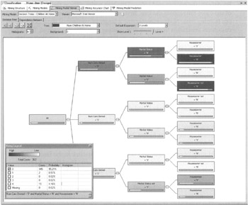
Figure 13-18: The decision tree with 0 Children At Home versus 1 or More Children At Home

Judging by the background color and the histograms, we can see two leaf nodes contain the most customers with no children at home. These are the Homeowner = N node under Marital Status = N and the Homeowner = N node under Marital Status = Y. In Figure 13-18, one of these two nodes is highlighted. This is the node with the most customers with no children at home. The bottom of the Mining Legend window shows thepath through the decision tree to get to this node. This can also be thought of as the rule that defines this decision tree node. From this, we can see that someone who owns no cars, is unmarried, and does not own a home is likely to have no children at home.

Microsoft Tree Viewer—Dependency Network Tab

Switching to the Dependency Network tab brings up a screen similar to Figure 13-19. This screen shows how each of the attributes included in the data mining model affect the other attributes. We can see which attributes predict other attributes. We can also see the strength of these interactions.

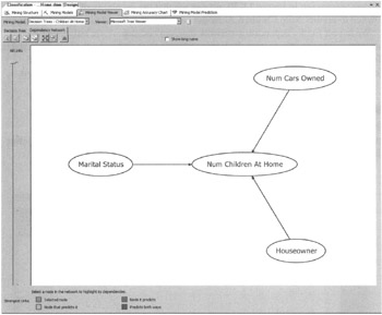
Figure 13-19: The Dependency Network tab for the Microsoft Decision Tree algorithm

Clicking on an attribute activates the color coding on the diagram. The selected node is highlighted with an aqua-green. The attributes predicted by the selected attribute are blue. The attributes that predict the selected attribute are light brown. If an attribute is predicted by the selected attribute, but also can predict that attribute, it is shown in purple. The key for these colors is shown below the diagram.

The arrows in Figure 13-19 also show us which attributes predict other attributes. The arrow goes from an attribute that is a predictor to an attribute it predicts. Num Cars Owned, Marital Status, and Houseowner all predict Num Children At Home.

The slider to the left of the diagram controls which arrows are displayed. When the slider is at the top, as shown in Figure 13-19, all arrows are visible. As the slider moves down, the arrows signifying weaker influences disappear. Only the stronger influences remain. In Figure 13-20, we can see that the capability of the Num Cars Owned to predict Num Children At Home is the strongest influence in the model.

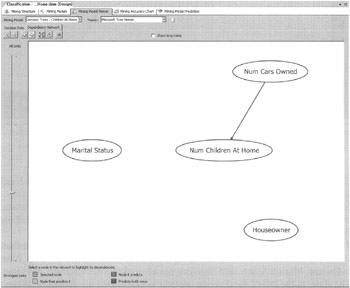
Figure 13-20: The strongest influence in this data mining model

We have a simple dependency network diagram because we are only using a few attributes. It is possible to have diagrams with tens or even hundreds of attribute nodes. To aid in finding a node in such a cluttered diagram, the viewer provides a search feature. To use the search feature, click the Find Node button (the binoculars icon).

Microsoft Mining Content Viewer

If, for some reason, we need to see the detailed data underlying the diagrams, it is available using the Microsoft Mining Content Viewer. This is selected using the Viewer drop-down list. The Microsoft Mining Content Viewer is shown in Figure 13-21.

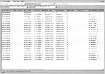
Figure 13-21: The Microsoft Mining Content Viewer

Microsoft Naïve Bayes

We look next at the tools available for reviewing the results of the Naïve Bayes algorithm. Recall, from Chapter 12, the Naïve Bayes algorithm deals only with the influence of each individual attribute on the predictable value. Let's see how this is represented graphically.

Microsoft Naïve Bayes Viewer—Dependency Network

Selecting the Naïve Bayes - Children At Home mining model from the Mining Model drop-down list displays the Microsoft Naïve Bayes Viewer - Dependency Network. This looks a lot like the Dependency Network Viewer we just looked at for the Decision Trees algorithm, as shown in Figure 13-22. (Does this look like a Klingon starship to you, too?) In fact, it functions in an identical manner. Using the slider to the left of the diagram, we can see the Num Cars Owned attribute is also the best predictor of Num Children At Home for this model. This is shown in Figure 13-23.

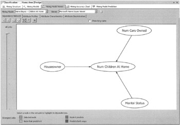
Figure 13-22: The Dependency Network Viewer for the Microsoft Naïve Bayes algorithm

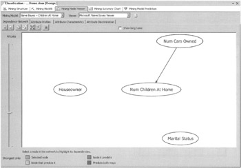
Figure 13-23: The strongest influence in this mining model

Attribute Profiles

Next, select the Attribute Profiles tab. We can select the predictable we want to analyze using the Predictable drop-down list. Num Children At Home is our only predictable in this model, so it is already selected. The diagram shows the distribution of each attribute value for the various predictable values. This is shown in Figure 13-24.

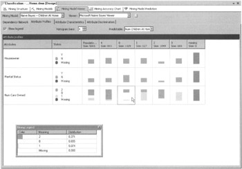
Figure 13-24: The Attribute Profiles Viewer for the Microsoft Naïve Bayes algorithm

Again, we have a Mining Legend window to provide more detailed information. Selecting a cell in the Attribute Profiles grid shows, in the Mining Legend, the numbers that underlie the histogram for that cell. The cell for the Num Cars Owned where Num Children At Home is 0 is selected and pointed to by the mouse cursor in Figure 13-24.

Attribute Characteristics

Select the Attribute Characteristics tab. Num Children At Home is already selected in the Attribute drop-down list and 0 is already selected in the Value drop-down list. We can see the attribute characteristics for the model. In other words, we can see the probability of a particular attribute value being present along with our predictable value. This is shown in Figure 13-25.

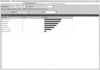
Figure 13-25: The Attribute Characteristics Viewer for the Microsoft Naïve Bayes algorithm

In this figure, we can see a customer with no cars has a high probability of having no children at home. We can also see a high probability exists that a customer who is not married does not have any children at home. There is a low probability that a person with one car has no children at home.

Attribute Discrimination

Select the Attribute Discrimination tab. Num Children At Home is already selected in the Attribute drop-down list and 0 is already selected in the Value 1 drop-down list. All Other States is selected in the Value 2 drop-down list. This diagram lets us determine what attribute values most differentiate nodes favoring our desired predictable state from those disfavoring our predictable. This is shown in Figure 13-26.

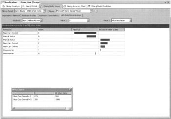
Figure 13-26: The Attribute Discrimination Viewer for the Microsoft Naïve Bayes algorithm

From the figure, we can see that not owning a car favors having no children at home. Being married favors having children at home. As with the other diagrams, selecting cell displays the detail for that cell in the Mining Legend.

Microsoft Clustering

We move from Naïve Bayes to the Microsoft Clustering algorithm. In Chapter 12, we learned the clustering algorithm creates groupings or clusters. We examine the clusters to determine which ones have the most occurrences of the predictable value we are looking for. Then we can look at the attribute values that differentiate that cluster from the others.

Cluster Diagram

Selecting the Clustering - Children At Home mining model from the Mining Model drop-down list displays the Microsoft Cluster Viewer - Cluster Diagram. We can see the algorithm came up with eight different clusters. The lines on the diagram show how closely related one cluster is to another. A dark gray line signifies two clusters that are strongly related. A light gray line signifies two clusters that are weakly related.

Select Num Children At Home from the Shading Variable drop-down list. The State drop-down list should have the 0 value selected. The shading of the clusters now represents the number of customers with 0 children at home in each cluster. This is shown in Figure 13-27.

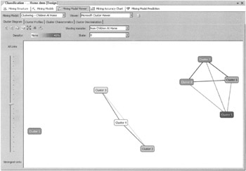
Figure 13-27: The Cluster Diagram Viewer for the Microsoft Clustering algorithm

In the diagram, Cluster 5 has the highest concentration of customers with no children at home. To make analysis easier on the other tabs, let's rename this cluster. Right-click Cluster 5 and select Rename Cluster from the Context menu. The Rename Cluster dialog box appears. Enter No Children At Home and click OK.

Cluster Profiles

Selecting the Cluster Profiles tab displays a grid of cluster profiles as shown in Figure 13-28. This functions exactly the same as the Naïve Bayes Attribute Profiles tab. We use this tab to examine the characteristics of the clusters that most interest us. In this case, it is easy to pick out the cluster of interest because we named it No Children At Home.

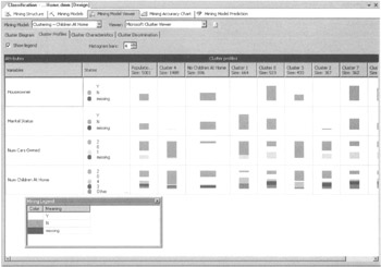
Figure 13-28: The Cluster Profiles Viewer for the Microsoft Clustering algorithm

Cluster Characteristics

We next select the Cluster Characteristics tab to display the grid of cluster characteristics. Select No Children At Home from the Cluster drop-down list to view the characteristics of this cluster. The Cluster Characteristics tab functions in the same manner as the Attribute Characteristics tab we encountered with the Microsoft Naïve Bayes algorithm. The Cluster Characteristics tab is shown in Figure 13-29.

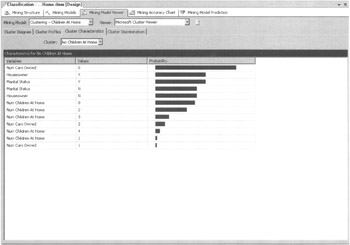
Figure 13-29: The Cluster Characteristics Viewer for the Microsoft Clustering algorithm

Cluster Discrimination

Select the Cluster Discrimination tab, and then select No Children At Home from the Cluster I drop-down list. This diagram enables us to determine what attribute values most differentiate our selected cluster from all the others. This is shown in Figure 13-30.

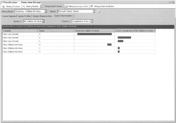
Figure 13-30: The Cluster Discrimination Viewer for Microsoft Clustering algorithm

Microsoft Neural Network

Selecting the Neural Network - Children At Home mining model from the Mining Model drop-down list displays the Microsoft Neural Network Viewer. The Microsoft Neural Network algorithm uses a Discrimination Viewer similar to those we have seen with other algorithms. This lets us determine the characteristics that best predict our predictable value.

Num Children At Home is already selected in the Output Attribute drop-down list. Select 0 in the Value 1 drop-down list. Select 1 in the Value 2 drop-down list. We can now see what differentiates customers with no children at home from customers with one child at home. The Discrimination Viewer is shown in Figure 13-31.

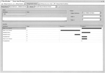
Figure 13-31: The Discrimination Viewer for the Microsoft Neural Network algorithm

Microsoft Association

The Microsoft Association algorithm deals with items that have been formed into sets within the data. In the example here, we look at sets of products that were purchased by the same customer. The Business Intelligence Development Studio provides us with three viewers for examining these sets.

Note 

We did not use the Microsoft Association or the other algorithms that follow in the remainder of this section in our mining structure.

Itemsets

The Itemsets Viewer is shown in Figure 13-32. The Itemsets Viewer shows a textual description of each set. The Support column shows the number of cases supporting the set. For clarity of analysis, we set Minimum Support to require at least 300 occurrences for a set to be displayed. The Size column tells us the number of members in the set.

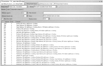
Figure 13-32: The Itemsets Viewer for the Microsoft Association algorithm

Rules

The Rules Viewer displays the rules the algorithm created from the sets. This is shown in Figure 13-33. The Probability column shows the probability of a rule being true. In Figure 13-33, we have a number of rules with a 100% probability—a sure thing! This means we do not have a single case in our training data set where this rule is not true.

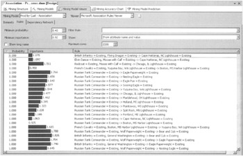
Figure 13-33: The Rules Viewer for the Microsoft Association algorithm

The Importance column tells us how useful the rule may be in making predictions. For example, if every set contained a particular attribute state, a rule that predicts this attribute state is not helpful; it is of low importance. The Rule column, of course, describes the rule. The rule at the top of Figure 13-33 says a set that contains a British Infantry figure and a Flying Dragon figure also contains a Cape Hatteras, NC Lighthouse.

Dependency Network

The Dependency Network Viewer functions in the same manner as we have seen with other algorithms. There is a node for each predictable state. In our example, there is a node for each member of the Product dimension. Selecting a product node shows which products it predicts will be in the set and which products predict it will be in the set. The Dependency Network Viewer is shown in Figure 13-34.

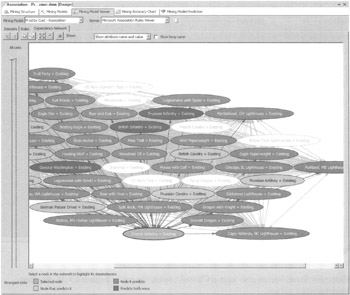
Figure 13-34: The Dependency Network Viewer for the Microsoft Association algorithm

Microsoft Sequence Clustering

The Microsoft Sequence Clustering algorithm is similar to the Microsoft Clustering algorithm. Consequently, these two algorithms use the same viewers. The only difference is the addition of the State Transitions Viewer. This viewer shows the probability of moving from one state in the sequence to another.

Microsoft Time Series

The Microsoft Time Series algorithm uses a Decision Tree Viewer, as we have seen with other algorithms. Recall from Chapter 12, each node in the decision tree contains a regression formula that is used to forecast future continuous values. The Microsoft Time Series also uses a Chart Viewer, shown in Figure 13-35, to chart these forecast values.

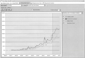
Figure 13-35: The Chart Viewer for the Microsoft Time Series algorithm