2.8. Shape Matching

As the availability of 3D models on the Internet and in databases increases , searching for such models becomes an interesting problem. Such a functionality is needed, for instance, in medical image databases or CAD databases. One question is how to specify a query. Usually, most researchers pursue the query by content approach, where a query is specified by providing a (possibly crude) shape, for which the database is to return best matches. ^[3] The fundamental step here is the matching of shapes ; i.e., the calculation of a similarity measure.

Almost all approaches perform the following steps:

Define a transformation function that takes a shape and computes a so-called feature vector in some high-dimensional space, which (hopefully) captures the shape in its essence. Naturally, those transformation functions that are invariant under rotation and/or translation and tessellation are preferred;
Define a similarity measure d on the feature vectors, such that if d ( f ₁ , f ₂ ) is large, then the associated shapes s ₁ , s ₂ do not look similar. Obviously, this is (partly) a human factor issue. In almost all algorithms, d is just the Euclidean distance;
Compute a feature vector for each shape in the database and store the vectors in a data structure that allows for fast nearest -neighbor search;
Given a query (a shape), compute its feature vector and retrieve the nearest neighbor from the database. Usually, the system also retrieves all k nearest neighbors. Often, you are not interested in the exact k nearest neighbors but only in approximate nearest neighbors (because the feature vector is an approximation of the shape anyway).

The main difference among most shape-matching algorithms is, therefore, the transformation from shape to feature vector.

So, fast shape retrieval essentially requires a fast (approximate) nearest-neighbor search. We could stop our discussion of shape matching here, but for sake of completeness, we will describe a very simple algorithm (from the plethora of others) to compute a feature vector [Osada et al. 01].

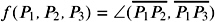
The general idea is to define some shape function f ( P ₁ , , P _n ) , which computes some geometrical property of a number of points, and then evaluate this function for a large number of random points that lie on the surface of the shape. The resulting distribution of f is called a shape distribution .

For the shape function, there are a lot of possibilities (your imagination is the limit). There are some examples:

f ( P ₁ , P ₂ ) = P ₁ ˆ P ₂ ,
f ( P ₁ ) = P ₁ ˆ P , where P is a fixed point, such as the bounding box center,
,
f ( P ₁ , P ₂ , P ₃ , P ₄ ) = volume of the tetrahedron between the four points.

Figure 2.15 shows the shape distributions of a few simple objects with the distance between two points as shape function.

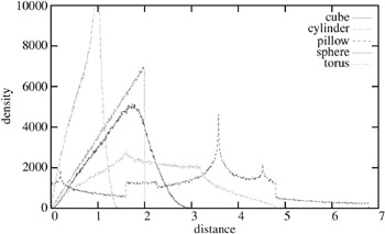
Figure 2.15: The shape distributions of a number of different simple objects. (See Color Plate XX.)

^[3] This idea seems to originate from image database retrieval, where it was called QBIC, for query by image content.