Chapter 3: BSP Trees

Overview

Binary space partitioning (BSP) trees can be viewed as a generalization of kd-trees. Like kd-trees , BSP trees are binary trees, but now the orientation and position of a splitting plane can be chosen arbitrarily. To get a feeling for a BSP tree, Figure 3.1 shows an example for a set of objects.

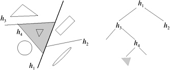
Figure 3.1: An example of a BSP tree for a set of objects.

The definition of a BSP (short for BSP tree) is fairly straightforward. Here, we will present a recursive definition. Let h denote a plane in , and h ⁺ and h ^ˆ denote the positive and negative half-space, respectively.

Definition 3.1. (BSP tree.)   Let S be a set of objects (points, polygons, groups of polygons, or other spatial objects), and let S ( ) denote the set of objects associated with a node . Then the BSP T ( S ) is defined by the following.

1. If S ‰ 1, then T is a leaf which stores S ( ) := S .

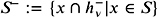
2. If S > 1, then the root of T is a node ; stores a plane h and a set S ( ) := { x ˆˆ S x h } (this is the set of objects that lie completely inside h ; in 3D, these can be only polygons, edges, or points). also has two children T ^ˆ and T ⁺ ; T ^ˆ is the BSP for the set of objects , and T ⁺ is the BSP for the set of objects .

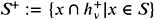This can readily be turned into a general algorithm for constructing BSPs. Note that a splitting step (i. e., the construction of an inner node) requires us to split each object into two disjoint fragments if it straddles the splitting plane of that node. In some applications though (such as ray shooting), this is not really necessary; instead, we can just put those objects into both subsets .

Note that a convex cell (which is possibly unbounded) is associated with each node of the BSP. The cell associated with the root is the whole space, which is convex. Splitting a convex region into two parts yields two convex regions . In Figure 3.1, the convex region of one of the leaves has been highlighted as an example.

With BSPs, we have much more freedom to place the splitting planes than with kd-trees. However, this also makes that decision much harder (as almost always in life). If our input is a set of polygons, then a very common approach is to choose one of the polygons from the input set and use this as the splitting plane. This is called an auto-partition (see Figure 3.2).

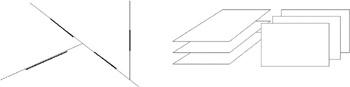
Figure 3.2: Left: an auto-partition. Right: an example of a configuration in which any auto-partition must have quadratic size .

While an auto-partition can have ( n ² ) fragments, it is possible to show the following in 2D [de Berg et al. 00, Paterson and Yao 90].

Lemma 3.2. Given a set S of n line segments in the plane, the expected number of fragments in an auto-partition T ( S ) is in O ( n log n ) . It can be constructed in time O ( n ² log n ) .

In higher dimensions, it is not possible to show a similar result. In fact, one can construct sets of polygons such that any BSP (not just auto-partitions) must have ( n ² ) many fragments (see Figure 3.2 for a bad example for auto-partitions).

However, all of these examples producing quadratic BSPs violate the principle of locality : polygons are small compared to the extent of the whole set. In practice, no BSPs have been observed that exhibit the worst-case quadratic behavior [Naylor 96].