2.7. Texture Synthesis

Textures are visual details of the rendered geometry. Textures have become very important in the past few years because the cost of rendering with texture is the same as the cost without texture. Virtually all real-world objects have texture, so it is extremely important to render them in synthetic worlds , too.

Texture synthesis generally tries to synthesize new textures, from given images, from a mathematical description, or from a physical model. Mathematical descriptions can be as simple as a number of sine waves to generate water ripples. Physical models try to describe the physical or biological effects and phenomena that lead to some texture (such as patina or fur). In all of these model-based methods, the knowledge about the texture is in the model and the algorithm. The other class of methods starts with one or more images, tries to find some statistical or stochastic description (explicitly or implicitly) of these, and finally generates a new texture from the statistic.

Basically, textures are images with the following properties:

Stationary: if a window with the proper size is moved about the image, the portion inside the window always appears the same;
Local: each pixels color in the image depends on only a relatively small neighborhood.

Of course, images not satisfying these criteria can be used as textures as well (such as faades), but if you want to synthesize such images, a statistical or stochastic approach is probably not feasible .

In the following, we will describe a stochastic algorithm that is very simple and efficient, and works remarkably well [Wei and Levoy 00]. Given a sample image, it does not, like most other methods, try to compute explicitly the stochastic model. Instead, it uses the sample image itself, which implicitly contains that model already.

We will use the following terminology:

Initially, T is cleared to black. The algorithm starts by adding a suitably sized border at the left and the top, filled with random pixels (this will be thrown away again at the end). Then it performs the following simple loop in scan line order (see Figure 2.12):

 1:  for all   p     T   do  2:         find the  p  _i    I  that minimizes  N  (  p  )    N  (  p  _i ) ² 3:  p  :=  p  _i 4:  end for

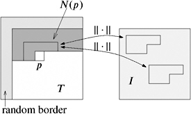
Figure 2.12: The texture synthesis algorithm proceeds in scan line order through the texture and considers only the neighborhood around the current pixel as shown.

The search in line 2 is exactly a nearest -neighbor search! This can be performed efficiently with the algorithm presented in Section 6.4.1: if N ( p ) contains k pixels, then the points are just 3 k -dimensional vectors of RGB values, and the distance is just the Euclidean distance.

Obviously, all pixels of the new texture are deterministically defined, once the random border has been filled. The shape of the neighborhood N ( p ) can be chosen arbitrarily; it must just be chosen such that all pixels but the current pixel are already computed. Likewise, other scans of the texture are possible and sensible (for instance, a spiral scan order); they must just match the shape of N ( p ).

The quality of the texture depends on the size of the neighborhood N ( p ). However, the optimal size itself depends on the granularity in the sample image. In order to make the algorithm independent, we can synthesize an image pyramid (see Figure 2.13). First, we generate a pyramid I , I ¹ , , I ^d for the sample image I . Then we synthesize the texture pyramid T , T ¹ , , T ^d level by level with the above algorithm, starting at the coarsest level. The only difference is that we extend the neighborhood N ( p ) of a pixel p over k levels, as depicted by Figure 2.13. Consequently, we have to build a nearest-neighbor search structure for each level, because as we proceed downwards in the texture pyramid, the size of the neighborhood grows.

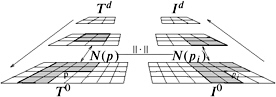
Figure 2.13: Using an image pyramid, the texture synthesis process becomes fairly robust against different scales of detail in the sample images.

Of course, now we have replaced the parameter of the best size of the neighborhood by the parameter of the best size per level and the best number of levels to consider for the neighborhood. However, as Wei and Levoy [Wei and Levoy 00] report, a neighborhood of 9 — 9 (at the finest level) across two levels seems to be sufficient in almost all cases.

Figure 2.14 shows two examples of the results that can be achieved with this method.

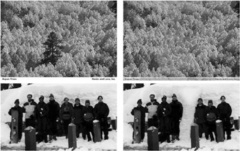
Figure 2.14: Some results of the texture synthesis algorithm [Wei and Levoy 00]. In each pair, the image on the left is the original one, and the one on the right is the (partly) synthesized one. (See Color Plate IV.) (Courtesy of L.-Y. Wei and M. Levoy, and ACM.)